Introduction
Lorem ipsum dolor sit amet, consetetur sadipscing elitr, sed diam nonumy eirmod tempor invidunt ut labore et dolore magna aliquyam erat, sed diam voluptua. At vero eos et accusam et justo duo dolores et ea rebum. Stet clita kasd gubergren, no sea takimata sanctus est Lorem ipsum dolor sit amet. Lorem ipsum dolor sit amet, consetetur sadipscing elitr, sed diam nonumy eirmod tempor invidunt ut labore et dolore magna aliquyam erat, sed diam voluptua. At vero eos et accusam et justo duo dolores et ea rebum. Stet clita kasd gubergren, no sea takimata sanctus est Lorem ipsum dolor sit amet.
math, optimization, julia, 90-01, 90C30
Why learn Optimization?
Convex optimisation is an important field of applied mathematics. It involves finding the minimum of a given objective function subject to certain constraints. Optimisation has many applications in machine learning, computational physics, and finance. Examples include minimising risk for portfolio optimisation, minimising an error function to fit a machine learning model and minimising the energy of a system in computational physics.
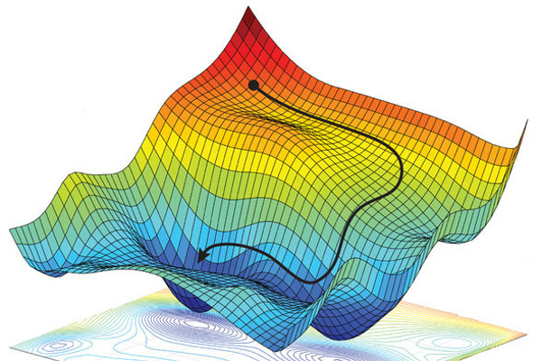
source: arXiv:1805.04829
About this Course
Target Audience
This course is primarily aimed at undergraduate students of mathematics, physics and engineering. However, it is also suitable for software developers and engineers interested in machine learning who want to develop a better understanding of the optimisation algorithms behind these models.
Prerequisites
This is not an introductory course, so a solid understanding of linear algebra and calculus. For the implementation of the numerical algorithms, it is also useful to have some programming skills in either MATLAB, Python or Julia. However, there will be a short introduction to Julia programming at the beginning, so basic programming skills are sufficient.
Syllabus
- Week 1 – 5: lorem ipsum
- Week 6 – 10: lorem ipsum
The exact structure of this course is subject to change and may vary.
Literature
Recommended Textbooks
The book [1] is certainly considered the ‘bible’ of convex optimisation. It has been cited over 4,400 times and is extremely comprehensive. The fact that it is available for free is an added bonus. However, I think this book is a bit overwhelming, especially for beginners. For instance, it devotes over 300 pages to the theory behind convex functions before moving on to numerical algorithms.
In my opinion, the book [2] by Nocedal and Wright is better structured, covering everything from quasi-Newton and trust region methods to algorithms for constrained optimisation problems.
Mathematical optimisation is a highly practical field. As such, a modern textbook on the subject should include code to demonstrate how to implement these algorithms in practice. This is the case for [3], which is an excellent textbook for bridging the gap between maths and programming. It also contains many colourful illustrations, making it a pleasure to read. If I had to recommend one book for learning optimization, it would be this one.
![[1]](images/literature/Convex_Optimization-Boyd.jpg)
![[2]](images/literature/Numerical_Optimization-Nocedal.jpg)
![[4]](images/literature/Nichtlineare_Optimierung.jpg)
![[3]](images/literature/Algorithms_for_Optimization.jpg)
Online Courses
There are also a few online courses on optimisation available. For example:
- Stanford EE364A Convex Optimization by Stephen Boyd, 2023
- Optimization Method for Machine Learning by Julius Pfrommer, KIT 2020/21
Introduction
This course focuses on optimisation problems of the following form:
Find a minimum of \[ \mathop{\mathrm{arg\,min}}_{\mathbf{x}} \; f(\mathbf{x}) \] subject to \[ \begin{aligned} h(\mathbf{x}) &= 0 \\ g(\mathbf{x}) &\leq 0 \end{aligned} \]
The function \(f\) is called objective function, and \(h\) and \(g\) are constraints of the optimization problem.
. . .
Such optimisation problems can arise, for example, from modelling real-world problems with neural networks, where the aim is to minimise the error between the model and the training dataset. However, large neuronal networks can have billions of parameters (‘weights’). Consequently, these problems can be extremely complex, to the extent that they cannot be solved by hand. We are therefore interested in finding algorithms that can solve these optimization problems efficiently.
. . .
A good optimisation algorithm should have the following properties:
- Robustness: The algorithm should work with a very general set of data.
- Efficiency: It should not require excessive computational resources.
- Accuracy: The results should be accurate and not overly sensitive to errors in the data.
Examples for Optimization Problems
Optimisation problems occur in all kinds of applications. Here are some examples:
1. Machine Learning
A common problem in machine learning is classification. You are given a set of points belonging to different classes and need to find a decision boundary to separate them. One possible solution is to fit the decision boundary so that the margin is maximised. This is the approach used by so-called Support Vector Machines (SVM).
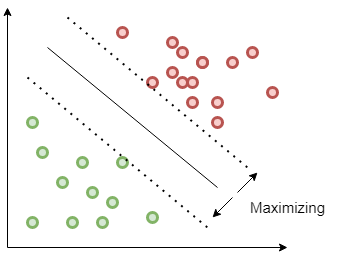
author: Sidharth GN, source: quarkml.com
If \(w\) is the normal vector of the decision boundary, \(b\) is the ‘bias’ parameter that determines the distance to the origin of the coordinate system and \(t_n\) is the target value (1 if the point \(x_n\) belongs to the class and -1 if it does not), then we need to find:
\[ \mathop{\mathrm{arg\,max}}_{\mathbf{w}, b} \frac{1}{\lVert \mathbf{w} \rVert} \min_{n=1,\dotsc,N} \left\{ t_n \mathbf{w}^\mathrm{T} \mathbf{x}_n + b \right\} \]
. . . Without loss of generality, we can choose w and b so that the margin is scaled to 1. This leads to the following optimization problem:
\[ \begin{aligned} \mathop{\mathrm{arg\,min}}_{\mathbf{w}, b} \frac{1}{2} \lVert \mathbf{w} \rVert^2 \\ \text{s.t.}\quad t_n (\mathbf{w}^\mathrm{T} \mathbf{x}_n + b) \geq 1 \end{aligned} \]
. . .
This is an example for a quadratic programming problem, which is quite difficult to solve.
2. Markowitz-Portfolio Optimization
The Markowitz Mean-Variance Portfolio Optimization model provides a framework for investors to construct diversified portfolios that minimize risk for a given level of expected return. The core idea is that investors care about two things: the expected return of their portfolio and the risk of that portfolio. By quantifying these, an optimal trade-off can be found.
This can be expressed mathematically as follows: Minimize the risk \[ \min_{\mathbf{x}} \mathbf{x}^\mathrm{T} \Sigma \mathbf{x} \]
. . .
subject to the constraints that the expected return exceeds a target value \(R_{\text{target}}\) and that the sum of all portfolio weights is 100%.
\[ \begin{aligned} \sum_{i=1}^N x_i &= 1 \\ \sum_{i=1}^N \mathbb{E}[R_i] x_i &\geq R_{\text{target}}. \end{aligned} \]
. . .
where:
- \(\mathbf{x}\) is a vector of portfolio weights between 0 and 100%,
- \(\Sigma\) is the covariance matrix representing the expected risk,
- \(\mathbb{E}[R_i]\) are the expected returns of each assets, and
- \(R_{\text{target}}\) is a constraint for the expected return
. . .
The risk of an asset is essentially its standard deviation in pricing, or its volatility. The covariance matrix and expected returns are model parameters that need to be estimated beforehand.
As the objective function is a quadratic form with a positive semi-definite covariance matrix, this is a convex optimisation problem.
3. Partial Differential Equations
The Poisson equation is one of the simplest differential equations. It describes the electric potential in a capacitor with a given charge density.
\[ \begin{aligned} - \Delta u &= f, && \text{in $\Omega$}, \\ u &= 0, && \text{on $\partial\Omega$} \end{aligned} \]
. . .
Here, \(\Omega := [a, b]^2 \subseteq \mathbb{R}^2\) is the domain of the problem, and \(u = 0\) is the (Dirichlet) boundary condition.
. . .
Multiplying both sides by a test function v and then applying Green’s identity gives us the weak formulation of the differential equation:
\[ \int_\Omega \nabla u \cdot \nabla v \, \mathrm{d}\mathbf{x} = \int_\Omega f v \,\mathrm{d}x \]
. . .
The weak formulation plays an important role in the finite element method. It can also be viewed as the Gateaux differential of an energy functional:
\[ J[u] = \frac{1}{2} \int_\Omega \nabla u \cdot \nabla u \, \mathrm{d}\mathbf{x} - \int_\Omega f v \,\mathrm{d}\mathbf{x} \overset{\text{!}}{=} \min \]
This is a variational problem. The minimum of the energy functional is also a solution of the Poisson equation.