Julia Basics
Julia is a modern programming language commonly used for numerical analysis and scientific computing. It combines the speed of languages like C++ or Fortran with the ease of use of Matlab or Python. In this tutorial I will show you how to program in Julia. We will cover types, collections and a very powerful feature called multiple dispatch. But for now, let us start with the basics.
julia, programming, scientific computing
Why Julia?
![]()
author: Stefan Karpinski
source: github.com
license: CC BY-NC-SA 4.0
Julia is a modern programming language that is commonly used for numerical analysis and scientific computing. It combines the speed of languages like C++ or Fortran with the ease of use of Matlab or Python. This is because Julia was designed to solve the “two-language problem”: A lot of software is often developed in a dynamic language like Python and then re-implemented in a statically typed language for better performance. With Julia, you get the best of both worlds:
Julia walks like Python, and runs like C++.
Literature
Recommended Textbooks
Julia is still a relatively new programming language, so there are few good books about it, and most of them are completely out of date. However, I can recommend the books “Julia as a Second Language” and “Julia for Data Analysis”, both of which give a really good introduction to Julia programming. The latter also has a large chapter on dataframes, which is definitely useful in data science. The book “Think Julia” also seems to be good, although a little less comprehensive.
![[1]](images/literature/Julia_as_a_Second_Language.jpg)
![[2]](images/literature/Julia_for_Data_Analysis.jpg)
![[3]](images/literature/Think_Julia.jpg)
![[4]](images/literature/Julia_Data_Science.png)
The best resources for learning Julia is definitely the Official Documentation, which is freely available on the Internet. Another course that is really really great is Julia for Optimization and Learning by the university of Prague. It gives a good introduction to Julia with examples from optimization and machine learning.
There is also a free Course on Coursera that should be mentioned. However, since I haven’t taken it, I can’t say whether it’s good or bad. It’s kinda okay; not good, not bad.
Other Resources:
- Official Documentation
- Course Julia for Optimization and Learning by the University of Prague
- Quantitative Economics with Julia by Jesse Perla, Thomas J. Sargent, and John Stachurski
- Lecture Computational Thinking, MIT 18.S191/6.S083
- Introducing Julia on WikiBooks
This course is fairly fast-paced.
It is assumed that the reader is already familiar with a programming language such as MATLAB, Python or C++.
I will be making comparisons to these languages throughout the course.
Getting Started
Let’s start with a simple hello-world. The print function works exactly like it does in Python:
print("Hello World!")
print("The answer is ", 42)
There is also the println() command, which is exactly the same except that it ends with a newline character.
println("Hello World!")Basic Math
Of course, you can use Julia like a calculator:
julia> 5 + 3
8

julia> 4 * 5
20

julia> 0.5 * (4 + 7)
5.5
. . .
Note that division implicitly converts the input into float; if you want to do integer division, use div(n, m).
julia> 11 / 7
1.5714285714285714

julia> div(11, 7)
1
>>> 11 / 7
1.5714285714285714
>>> 11 // 7
1. . .
To calculate the power of a number, use the ^ operator (similar to Matlab):
julia> 2^4
16
>> 2^4
16>>> 2**4
16Julia provides a very flexible system for naming variables. In the Julia REPL, you can write mathematical symbols and other characters with a tab; for example, the Greek letter π can be typed via \pi<TAB>.
This makes it possible to translate mathematical formulas into code in a very elegant way.
julia> sin(π) ≠ 1/2
true

julia> √25
5.0
There are alot of built-in math functions:
julia> cos(pi)
-1.0

julia> sqrt(25)
5.0

julia> exp(3)
20.085536923187668

julia> rand()
0.8421147919589432
>> cos(pi)
ans = -1
>> sqrt(25)
ans = 5
>> exp(3)
ans = 20.08553692318767
>> rand()
ans = 0.2162824594661559>>> import numpy as np
>>> np.cos(np.pi)
-1.0
>>> np.sqrt(25)
5.0
>>> np.exp(3)
20.085536923187668
>>> np.random.rand()
0.8839348951868577. . .
You might be wondering what happens when you try to overwrite a built-in function or symbol:
julia> pi
π = 3.1415926535897...

julia> pi = 3
ERROR: cannot assign a value to imported variable Base.pi from module Main

julia> sqrt(100)
10.0

julia> sqrt = 4
ERROR: cannot assign a value to imported variable Base.sqrt from module Main
Dynamic Binding
Like Python, Julia is a dynamically typed language. This means that variables do not have a fixed data type like in C++, but can point to different data via dynamic binding.
Consider two variables, x and y. After assigning y to x, both variables point to the same memory location; no data is being copied.

This figure was created with draw.io and is hereby licensed under Public Domain (CC0 1.0)
In Python you can use the id() operator to see what’s actually going on:
>>> x = 42
>>> y = 3.7
>>> id(x)
11755208
>>> id(y)
134427599166672
>>> x = y
>>> x
3.7
>>> id(x)
134427599166672
int x = 42;
std::string str = "Hello!";
x = str; // Compile error!As you can see, after the assignment, both variables have the same memory address. Something like that would not be possible in C++.1
This distinction may seem trivial, but has some important implications when dealing with mutable types, whose contents can be changed:
a = [1, 2, 3]
b = a
a[2] = 42julia> b
3-element Vector{Int64}:
1
42
3>>> import numpy as np
>>> a = np.array([1, 2, 3])
>>> b = a
>>> a[1] = 42
>>> b
array([ 1, 42, 3]). . .
As no copy is being made, any change to variable a will also affect variable b. To actually make a deep copy, use the deepcopy() command2:
b = deepcopy(a)b = a.copy(). . .
For performance reasons, avoid binding values of different types to the same variable.
Code that avoids changing the type of a variable is called type stable.
Numbers in Julia
You can see the type of a variable with the typeof() operator:
julia> x = 42
42

julia> typeof(x)
Int64

julia> typeof(3.7)
Float64
>>> x = 42
>>> type(x)
<class 'int'>
>>> type(3.7)
<class 'float'>>> x = int64(42)
x = 42
>> y = 3.7
y = 3.7
>> whos
Variables visible from the current scope:
variables in scope: top scope
Attr Name Size Bytes Class
==== ==== ==== ===== =====
x 1x1 8 int64
y 1x1 8 double
Total is 2 elements using 16 bytes. . .
Julia uses 64 bits for integers and floats by default. Other types available are:
Int8, Int16, Int32, Int64, Int128, BigInt
UInt8, UInt16, UInt32, UInt64, UInt128
Float16, Float32, Float64, BigFloat
. . .
To define a variable of a given size, use x = int16(100). For example, to define an integer of arbitrary length, use
x = BigInt(1606938044258990275541962092341162602522202993782792835301376). . .
As specified in the IEEE754 standard, floating point numbers support inf and NaN values.
julia> -5 / 0
-Inf

julia> 0 * Inf
NaN

julia> NaN == NaN
false
>>> -5 / 0
Traceback (most recent call last):
File "<input>", line 1, in <module>
-5 / 0
~~~^~~
ZeroDivisionError: division by zero
>>> 0 * np.Inf
nan
>>> np.nan == np.nan
False>> -5 / 0
ans = -Inf
>> 0 * Inf
ans = NaN
>> NaN == NaN
ans = 0. . .
Floating point numbers can only be approximated, so a direct comparison using a==b may give unexpected results:
julia> 0.2 + 0.1 == 0.3
false

julia> 0.2 + 0.1
0.30000000000000004
>>> 0.2 + 0.1 == 0.3
False
>>> 0.2 + 0.1
0.30000000000000004>> 0.2 + 0.1 == 0.3
ans = 0
>> 0.2 + 0.1
ans = 0.3This is a general problem with floating point numbers, and exists in other programming languages as well.
. . .
The machine precision can be obtained with eps(), which gives the distance between 1.0 and the next larger representable floating-point value:
julia> eps(Float64)
2.220446049250313e-16
>> eps
ans = 2.220446049250313e-16. . .
Using that, we can implement a function isapprox(a, b) to test whether to numbers are approximately equal:
function isapprox(x::Real, y::Real; atol::Real=1e-14, rtol::Real=10*eps())
        return abs(x - y) <= atol + rtol * max(abs(x), abs(y))
end
. . .
Fortunately, such a function already exists in the standard library:
julia> isapprox(0.2 + 0.1, 0.3)
true

julia> 0.2 + 0.1 ≈ 0.3
true
>>> np.allclose(0.2 + 0.1, 0.3)
TrueNumerical Literal Coefficients
When multiplying variables with a coefficient, you can omit the multiplication symbol *.
julia> x = 3
3

julia> 2x^2 - 5x + 1
4
. . .
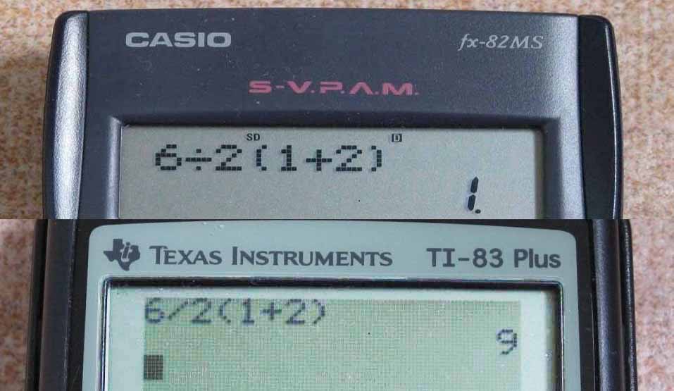
As a consequence, coefficients have a higher priority than other operations (“multiplications via juxtaposition”):
julia> 6 / 2x
1.0
. . .
Overflow Behaviour
As in other programming languages, exceeding the maximum representable value of a given type results in wraparound behaviour:
julia> n = typemax(Int64)
9223372036854775807

julia> n + 1
-9223372036854775808
In this sense, calculating with integers is always a form of modulo arithmetic.
Control Flow
Control structures such as branches and loops are easy to implement in Julia; the syntax is very similar to MATLAB:
if x > 0
  println("x is positive")
elseif x < 0
  println("x is negative")
else
  println("x is zero")
end
if x > 0
disp("x is positive")
elseif x < 0
disp("x is negative")
else
disp("x is zero")
endif x > 0:
print("x is positive")
elif x < 0:
print("x is negative")
else:
print("x is zero")if (x > 0) {
std::println("x is positive");
} else if (x < 0) {
std::println("x is negative");
} else {
std::println("x is zero");
}. . .
Just as in C++, Julia supports the ternary if statement:
println(x < y ? "less than" : "greater or equal")std::println(x < y ? "less than" : "not less than");. . .
Multiple logical conditions can be combined with basic comparison operators:
A && B    # A and B
A || B    # A or B
A != B    # A XOR B
. . .
Of course, logical operations do short-circuit evaluation:
julia> n = 2;

julia> n == 1 && println("n is one")
false
>>> n = 2
>>> n == 1 and print("n is one")
False>> n = 2;
>> n == 1 && disp("n is one")
ans = 0Loops
To iterate over a range or an array, use a for-each loop:
arr = ["Coffee", "Cocoa", "Avocado", "Math!"];

for item in arr
  println(item)
end
arr = ["Coffee", "Cocoa", "Avocado", "Math!"]
for item in arr:
print(item)auto arr = std::vector<std::string>{"Coffee", "Cocoa", "Avocado", "Math!"};
for (const auto& item : arr){
std::println(item);
}. . .
This can be used to iterate over a specific range:
for i in 1:4
  println(i)
end
for (int i = 1; i <= 4; ++i){
std::println(i);
}for i = 1:4
disp(i)
endfor i in range(1, 5):
print(i). . .
Of course, the same can be achieved with a while-loop:
i = 1

while i ≤ 4
  println(i)
  i += 1
end
i = 1
while i <= 4:
print(i)
i += 1i = 1
while i <= 4
disp(i)
i += 1;
endException Handling
Exceptions are a way of dealing with unexpected errors. When such an error occurs, it is best to deal with the problem as early as possible. By throwing an exception, you skip the entire function call until it reaches a point where the exception is caught.
. . .
For example, the sqrt function throws a DomainError when applied to a negative real value:
julia> sqrt(-1)
ERROR: DomainError with -1.0:
sqrt was called with a negative real argument but will only return a complex result if called with a complex argument. Try sqrt(Complex(x)).
Stacktrace:
[...]
>>> math.sqrt(-1)
Traceback (most recent call last):
File "<input>", line 1, in <module>
math.sqrt(-1)
ValueError: math domain error. . .
An exception like this can be thrown using the throw keyword:
if x <= 0
    err = DomainError(x, "`x` must be positive.")
    throw(err)
end
. . .
There are many built-in exceptions available.
| Exception |
|---|
| DomainError |
| ArgumentError |
| BoundsError |
| OverflowError |
. . .
You may also define your own exceptions in the following way:
julia> struct MyCustomException <: Exception end. . .
An error is an eception of type ErrorException. It can be used to interrupt the normal control flow.
julia> fussy_sqrt(x) = x >= 0 ? sqrt(x) : error("negative x not allowed")
fussy_sqrt (generic function with 1 method)
. . .
The try-catch block can be used to handle exceptions:
try
    # Code
catch e::DomainError
    # Handle specific error
catch
    # Handle other errors
end
Functions
Simple functions can be defined via:
f(x) = x^2f = lambda x: x**2auto f = [](auto x){ return x*x; };. . .
More advanced functions are defined using the function keyword:
function fac(n::Integer)
  @assert n > 0 "n must be positive"

  if n ≤ 1
    return 1
  else
    return n * fac(n-1)
  end
end
def fac(n: int) -> int:
assert n > 0, "n must be positive!"
if (n <= 1):
return 1
else:
return n * fac(n - 1)Note that we use the @assert macro to ensure that the arguments are positive.
. . .
Functions can be applied element-wise to arrays using the dot notation, f.(x):
julia> x = [0, 1, 2, 3, 4, 5];
julia> f(x) = x^2;
julia> f.(x)
6-element Vector{Int64}:
  0
  1
  4
  9
 16
 25
>>> import numpy as np
>>> x = np.array([-11, 1, 2, 3, 4, 5])
>>> f = lambda x: x**2
>>> f(x)
array([ 0, 1, 4, 9, 16, 25])>> x = [0, 1, 2, 3, 4, 5];
>> f = @(x) x.^2
f =
@(x) x .^ 2
>> f(x)
ans = 0 1 4 9 16 25. . .
The same can be achieved with the map(f, arr) function:
julia> map(f, x)
6-element Vector{Int64}:
  0
  1
  4
  9
 16
 25
. . .
The advantage of the map command is that it can also be applied to anonymous functions:
julia> map(x -> x^2, [0, 1, 2, 3, 4, 5])
6-element Vector{Int64}:
  0
  1
  4
  9
 16
 25
Optional Arguments
Functions in Julia can have positional arguments and keyword arguments, which are separated with a semicolon ;.
function f(x, y=10; a=1)
  return (x + y) * a
end
. . .
Such a function can be called via:
julia> f(5)
15

julia> f(2, 5)
7

julia> f(2, 5; a=3)
21
Varargs Functions
Sometimes it is convenient to write functions which can take an arbitray number of arguments. Such a function is called varargs functions. You can define a varargs function by following the last positional argument with an ellipsis:
function display(args...)
        println(typeof(args))
        for x in args
                println(x)
        end
endjulia> display(42, 3.7, "hello")
Tuple{Int64, Float64, String}
42
3.7
hellotemplate<typename... Args>
void display(Args&&... args)
{
(std::cout << ... << args) << '\n';
}42
3.7
hello. . .
Note that the varargs mechanism works differently in Julia than in C++. In C++, the expression args + ... is shorthand for recursion, meaning that the expression is evaluated to ((((x1 + x2) + x3) + x4) + ... ).
In Julia, however, it is much simpler: the varargs argument is just a tuple that you can iterate over.
Naming convention
As a convention in Julia, functions that modify an argument should have a ! at the end.
For example, sort() and sort!() both sort an array; however, one returns a copy, and the other functions sorts the array in place.
. . .
It is also good practice to use return nothing to indicate that a function does not return anything.
function do_something()
  println("Hello world!")
  return nothing
endImplement a function which calculates the sine of a real number x.
\[ \sin(x) = \sum_{k=0}^\infty (-1)^k \frac{x^{2k+1}}{(2k+1)!} \]
. . .
function sine(x::Real)
        @assert 0 <= x && x <= pi/4

        sine = 0.0
        for k in 0:9
                sine += (-1)^k * x^(2k + 1) / factorial(2k + 1)
        end
        return sine
end
Strings
One can think of a String as an array of characters with some convenience functions. Julia supports Unicode characters via the UTF-8 encoding.
. . .
As in Java and Python, strings are immutable. The value of a string object cannot be changed.
julia> name = "Markus"
"Markus"

julia> pointer_from_objref(name)
Ptr{Nothing} @0x000072d21dee95b8

julia> name = "Aurelius"
"Aurelius"

julia> pointer_from_objref(name)
Ptr{Nothing} @0x000072d21deea6c8
. . .
To change a character in a string, you have to first convert the string to an array, modify the desired character, and then join the array back into a string:
str = "hello world"
chars = collect(str)
chars[6] = '_'
new_str = join(chars)  # hello_world
str = "hello world"
char_list = list(str)
char_list[5] = '_'
new_str = ''.join(char_list)
print(new_str) # hello_worldSingle Characters
There is a class-type for single characters, AbstractChar:
julia> c = 'ü'
'ü': Unicode U+00FC (category Ll: Letter, lowercase)

julia> typeof(c)
Char
. . .
You can easily convert a character to its integer value:
julia> Int(c)
252
. . .
Keep in mind that not all integer values are valid unicode characters. For performance, the Char conversion does not check that every value is valid.
julia> Char(0x110000)
'\U110000': Unicode U+110000 (category In: Invalid, too high)

julia> isvalid(Char, 0x110000)
false
. . .
Since characters are basically like integers, you can treat them as such.
julia> 'A' < 'a'
true

julia> 'x' - 'a'
23
String Basics
String literals are delimited by double quotes (not single quotes):
julia> str = "Hello World!\n"
"Hello World!\n"

julia> str[begin]
'H': ASCII/Unicode U+0048 (category Lu: Letter, uppercase)

julia> str[end]
'\n': ASCII/Unicode U+000A (category Cc: Other, control)

julia> str[2:5]
"ello"
>>> str = "Hello World!\n"
>>> str[0]
'H'
>>> str[-1]
'\n'
>>> str[1:4]
'ell'Substrings
A SubString is a view into another string. It does not allocate memory, but instead references the original string.
# Range Indexing
str = "Hello, World!"
substring_copy = str[1:5]  # Creates a new string copy
println(substring_copy)  # Outputs: "Hello"

# SubString Function
str = "Hello, World!"
substring_view = SubString(str, 1, 5)  # Creates a view into the original string
println(substring_view)  # Outputs: "Hello"
. . .
So while both methods can extract a substring, the SubString function is more memory-efficient as it does not create a new string but rather a view into the original string.
Unicode and UTF-8
As mentioned above, Julia supports Unicode characters. Because of the variable length encodings, you cannot iterate over a string as you can in a normal array. Not every integer is a valid index.
julia> str  = "\u2200 x \u2203 y"
"∀ x ∃ y"

julia> str[1]
'∀': Unicode U+2200 (category Sm: Symbol, math)

julia> str[2]
ERROR: StringIndexError: invalid index [2], valid nearby indices [1]=>'∀', [4]=>' '
Stacktrace:
[...]

julia> str[4]
' ': ASCII/Unicode U+0020 (category Zs: Separator, space)
>>> str = "\u2200 x \u2203 y"
>>> str
'∀ x ∃ y'
>>> str[0]
'∀'
>>> str[1]
' '
>>> str[2]
'x'This also means that the number of characters in a string is not always the same as the last index.
julia> str
"∀ x ∃ y"

julia> length(str)
7   # number of characters

julia> lastindex(str)
11  # last index
. . .
To iterate through a string, you can use the string as an iterable object:
julia> for c in str
         print(c)
       end
∀ x ∃ y
. . .
If you need to obtain the valid indices for a string, you can use the eachindex function:
julia> collect(eachindex(str))
7-element Vector{Int64}:
  1
  4
  5
  6
  7
 10
 11
Concatenation
Multiple strings can be concatenated:
julia> str = "Hello " * "world"
"Hello world"
>>> str = "Hello " + "world"
>>> str
'Hello world'. . .
The choice of * to concatenate strings may seem unusual, but mathematically it makes sense, since concatenation is a non-commutative operation.
String Interpolation
You can evaluate variables within a string with the $ character:
julia> x = 42
42

julia> "The solution is $x"
"The solution is  42"

julia> "1 + 2 = $(1 + 2)"
"1 + 2 = 3"
Common String Operations
Basic string operations
julia> "Avocado" < "Coffee"
true

julia> findfirst("and", "Avocados and Chocolate and Coffee.")
10:12

julia> findall("and", "Avocados and Chocolate and Coffee.")
2-element Vector{UnitRange{Int64}}:
 10:12
 24:26
. . .
To repeat a string multiple times, use repeat:
>>> "...X" * 5
'...X...X...X...X...X'julia> repeat("...X", 5)
"...X...X...X...X...X". . .
Two other very handy operations are split and join:
julia> str = "Germany,Berlin,83500000,357596,+49,de"
"Germany,Berlin,83500000,357596,+49,de"

julia> words = split(str, ',')
6-element Vector{SubString{String}}:
 "Germany"
 "Berlin"
 "83500000"
 "357596"
 "+49"
 "de"

julia> join(words, ',')
"Germany,Berlin,83500000,357596,+49,de"
>>> str = "Germany,Berlin,83500000,357596,+49,de"
>>> words = str.split(',')
>>> words
['Germany', 'Berlin', '83500000', '357596', '+49', 'de']
>>> ','.join(words)
'Germany,Berlin,83500000,357596,+49,de'. . .
These functions are very useful for handling csv-data.
. . .
To check whether a string contains a specific substring, we can either use occursin or contains.
julia> occursin("world", "Hello world.")
true

julia> contains("Hello world.", "world")
true
For more complicated operations, it is recommended to use regular expressions.
Regular Expressions
Julia uses Perl-compatible regular expressions (regexes), as provided by the PCRE library.
Regular expressions are a common concept found in other programming languages, so there is no need to go into detail here. For a quick refresher, I refer the reader to the Python regex documentation and the tutorial on regular-expressions.info.
. . .
julia> re = r"^\s*(?:#|$)"
r"^\s*(?:#|$)"

julia> typeof(re)
Regex
>>> import re
>>> rx = re.compile(r'^\s*(?:#|$)')
>>> type(rx)
<class 're.Pattern'>. . .
For example, to match comment lines, you can use the following regex:
m = match(r"^\s*(?:#|$)", line)
if m === nothing
    println("not a comment")
else
    println("blank or comment")
end
m = re.match(r'^\s*(?:#|$)', line)
if m==None:
print("not a comment")
else:
print("blank or comment"). . .
Here is a simple regex to parse a string that contains the time:
julia> time = "12:45"
"12:45"

julia> m=match(r"(?<hour>\d{1,2}):(?<minute>\d{2})","12:45")
RegexMatch("12:45", hour="12", minute="45")
. . .
Write a regular expression to parse bibliography data in the following format:
surename, forename, and surename2, forename2. year. Title. Publisher.Example:
Lauwens, Ben, and Allen B. Downey. 2019. Think Julia. O’Reilly Media.. . .
julia> m = match(r"^(?P<names>.*)\. (?P<year>\d{4})\. (?<title>.*)\. (?<publisher>.*)\.$", str)
RegexMatch("Lauwens, Ben, and Allen B. Downey. 2019. Think Julia. O’Reilly Media.", names="Lauwens, Ben, and Allen B. Downey", year="2019", title="Think Julia", publisher="O’Reilly Media")

julia> authors = split(m["names"], " and ")
2-element Vector{SubString{String}}:
 "Lauwens, Ben,"
 "Allen B. Downey"

julia> year = parse(Int, m["year"])
2019
Pretty Output
Symbols
Symbols are a special type of immutable data that represent identifiers or names. They are denoted by a colon (:) followed by the name, such as :example.
The advantage of symbols over strings is that they offer very efficient comparisons:
julia> @btime "abcd" == "abcd"
  5.632 ns (0 allocations: 0 bytes)
true

julia> @btime :abcd == :abcd
  0.025 ns (0 allocations: 0 bytes)
true
In this sense, symbols are very similar to enums, except that they do not provide type safety: all symbols are of type “symbol”, whereas enums have their own distinct types.
Symbols are also used for meta-programming, which we will learn more about later.
Fixed-width Strings
In many data science applications we have to deal with strings that are only a few characters long. For example, city names are usually very short, and country codes are only two characters long.
For better performance, it is advantageous to store such data using a fixed-width string. This can be done using the InlineStrings.jl package, which provides eight fixed-width string types of up to 255 bytes.
julia> using InlineStrings

julia> country = InlineString("South-Korea")
"South-Korea"

julia> typeof(country)
String15
TODO: Move this to chapter 5.
Annotated Strings
Is is possible to store additional information inside a string by
julia> printstyled("WARNING!", color=:red, bold=true, blink=true)
WARNING!

julia> str = styled"{green:Avocados} are {bold:green}"
"Avocados are green"
References
Footnotes
It is possible to achieve this in C++ by using pointers or std::any, but let’s not go there.↩︎
see also on stackoverflow: Copy or clone a collection in Julia↩︎