---
title: "Fundamentals of Optimization"
author: "Marcel Angenvoort"
date: 2025-07-01
#doi: 10.5555/12345678
bibliography: "references.bib"
abstract: >
Lorem ipsum dolor sit amet, consetetur sadipscing elitr, sed diam nonumy eirmod tempor invidunt ut labore et dolore magna aliquyam erat, sed diam voluptua. At vero eos et accusam et justo duo dolores et ea rebum. Stet clita kasd gubergren, no sea takimata sanctus est Lorem ipsum dolor sit amet. Lorem ipsum dolor sit amet, consetetur sadipscing elitr, sed diam nonumy eirmod tempor invidunt ut labore et dolore magna aliquyam erat, sed diam voluptua. At vero eos et accusam et justo duo dolores et ea rebum. Stet clita kasd gubergren, no sea takimata sanctus est Lorem ipsum dolor sit amet.
keywords: ["math", "optimization", "julia", "90-01", "90C30"]
jupyter: julia-1.12
execute:
enabled: true
format:
html:
output-file: fundamentals_of_optimization.html
revealjs:
output-file: fundamentals_of_optimization-slides.html
# typst:
# output-file: fundamentals_of_optimization.pdf
---
Optimization Problems
----------------------
An Optimization problem in **standard form** is given by:
$$
\begin{aligned}
\text{minimize} &\quad f(\mathbf{x}) \\
\text{s.t.} \quad
\mathbf{h}(\mathbf{x}) &= 0 \\
\mathbf{g}(\mathbf{x}) &\leq 0
\end{aligned}
$$
. . .
We call $\mathbf{x}^\ast$ an **optimal point** if it solves the optimization problem, and $p^\ast$ is the corresponding **optimal value**.
. . .
Examples: (see notes 1)
- box constraints
- maximization problems
- equivalence of optimization problems
### Transforming the optimization problem
We can transform the optimization problem from the standard form
to the **epigraph form**:
$$
\begin{aligned}
\text{minimize} \quad &t \\
\text{s.t.} \quad
f(\mathbf{x}) - t &\leq 0 \\
\qquad \mathbf{g}(\mathbf{x}) &\leq \mathbf{0} \\
\qquad \mathbf{h}(\mathbf{x}) &= \mathbf{0}
\end{aligned}
$$
. . .
Geometrically, we can interpret this as an optimisation problem in 'graph space'. Find $x$ and $t$ such that $(x, t)$ belongs to the epigraph of $f$, and such that $x$ belongs to the feasible region.
```{julia}
#| label: fig-epigraph-form
#| fig-cap: "Optimization problem in Epigraph form"
using Plots
using LaTeXStrings
theme(:dark)

#default(size = (800, 600))  # set default plot size

# Define the function f(x)
f(x) = - 0.0457x^3 + 0.7886x^2 - 3.0857x + 5.5

# Define the x-range
x_range = 0:0.01:6

# Find the minimum point (x*, f(x*)) for the visualization
x_star = 2.5

# Create the plot
plot(x_range, f.(x_range),
    label = "f(x)",
    linewidth = 4,
    color = :black,
    xlabel = "x",
    ylabel = "t",
    title = "Optimization Problem in Epigraph Form",
    ylim = (0, 5.5),
    legend = false,
)

# Fill the area above the graph in blue to represent epi(f)
plot!(x_range, f.(x_range),
  fillrange = 5.5, fillalpha = 0.2, c = :blue, linealpha = 0)

# Add the label "epi(f)" in the middle of the blue area
annotate!(2.5, 4, text("epi(f)", :center, 20, :black))
annotate!(2.6, 1.9, text(L"(x^\ast, t^\ast)", :left, :top, :white, 20))

# Add the red point at (x*, f(x*))
scatter!([x_star], [f(x_star)],
    markersize = 8,
    markercolor = :red,
)
```
---
Consider the following optimization problem:
$$
\begin{aligned}
\text{minimize} \quad&f(\mathbf{x}_1, \mathbf{x}_2) \\
\text{subject to}\quad &\mathbf{g}(\mathbf{x_1}) \leq 0 \\
&\tilde{\mathbf{g}}(\mathbf{x_2}) \leq 0
\end{aligned}
$$
. . .
If we define the function $\tilde{f}$ via
$$
\tilde{f}(\mathbf{x}) := \inf \bigl\{ f(\mathbf{x}, \mathbf{z}) : \tilde{g}(\mathbf{z}) \leq \mathbf{0} \bigr\},
$$
. . .
then the optimization problem is equivalent to:
$$
\begin{aligned}
\text{minimize} \quad &\tilde{f}(\mathbf{x}) \\
\text{subject to} \quad &\mathbf{g}(\mathbf{x}) \leq 0
\end{aligned}
$$
. . .
Example: see notes 2.
### Convex Optimization
A convex optimization problem has the form:
$$
\begin{aligned}
\text{minimize}\quad &f(\mathbf{x}) \\
\text{s.t.} \quad &\mathbf{g}(\mathbf{x}) \leq 0 \\
&\mathbf{a}^\mathrm{T} \mathbf{x} = b
\end{aligned}
$$
where:
- the objective function $f$ is convex,
- the inequality constraints $\mathbf{g}$ are convex,
- the equality constraints $\mathbf{h}$ are affine
### Optimality criterion
Let
$$
X := \bigl \{ \mathbf{x} \in \mathbb{R}^n: \, \mathbf{g}(\mathbf{x}) \leq \mathbf{0}, \, \mathbf{h}(\mathbf{x}) = \mathbf{0} \bigr \}
$$
be the **feasible set**.
Then the following optimality criterion holds:
. . .
:::{.callout-important}
## Optimality Criterion
The point $x^\ast$ is an optimal point for the optimization problem if and only if
$$
\nabla f(\mathbf{x}^\ast) \cdot ( \mathbf{y} - \mathbf{x}^\ast ) \geq 0 \quad \forall \mathbf{y} \in X
$$
:::
::: {.proof}
See notes 3.
:::
### Linear Programming
A **linear program** is an optimization problem where the objective function is linear and the constraint functions are affine.
$$
\begin{aligned}
\text{minimize} \quad & \mathbf{c}^\mathrm{T} \mathrm{x} + \mathbf{d} \\
\text{s.t.} \quad& B\mathbf{x} \leq \mathbf{h}, \\
&A\mathbf{x} = \mathbf{b}
\end{aligned}
$$
. . .
By introducing a **slack variable** $s$, this can be transformed into a **linear program in standard form**:
. . .
$$
\begin{aligned}
\text{minimize} \quad \mathbf{c}^\mathrm{T} \mathbf{x} \\
\begin{aligned}
\text{s.t.} \quad
B\mathbf{x} + \mathbf{s} &= \mathbf{h} \\
A\mathbf{x} &= \mathbf{b} \\
\mathbf{s} &\geq \mathbf{0}
\end{aligned}
\end{aligned}
$$
### Quadratic Programming
The convex optimization problem is called a **quadratic program** (QP) if the objective function is quadratic, and the constraint functions are affine.
$$
\begin{aligned}
\text{minimize}\quad & \frac{1}{2} \mathbf{x}^\mathrm{T} P \mathbf{x} + \mathbf{q}^\mathrm{T} \mathbf{x} + r, \\
\text{subject to} \quad &\quad G\mathbf{x} \leq \mathbf{h} \\
&\quad A\mathbf{x} = \mathbf{b}
\end{aligned}
$$
. . .
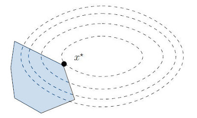
Visually, this means we are minimizing a quadratic function over a polyhedron.

license: [CC BY 4.0](https://creativecommons.org/licenses/by/4.0/)](images/quadratic_programming.jpg){#fig-quadratic-program width=50%}
. . .
A generalization of a quadratic program is the **quadratically constrained quadratic program** (QCQP):
$$
\begin{aligned}
\text{minimize}\quad & \frac{1}{2} \mathbf{x}^\mathrm{T} P \mathbf{x} + \mathbf{q}^\mathrm{T} \mathbf{x} + r, \\
\text{subject to} \quad& \frac{1}{2} \mathbf{x}^\mathrm{T} P_i \mathbf{x} + \mathbf{q}_i^\mathrm{T} \mathbf{x} + r_i \leq 0, \\
&\quad A\mathbf{x} = \mathbf{b}
\end{aligned}
$$
where $P_i$ are all symmetric positive definite.
. . .
Obviously, every quadratic program is also a QCQP.
### Example: Linear Regression
Linear regression leads to an over-determined linear system of equations
$A\mathbf{x} = \mathbf{b}$.
Finding the optimal solution is equivalent to minimizing the residual sum-of-sqares error
$$
E(\mathbf{x}) = \frac{1}{2} \lVert A\mathbf{x} - b \rVert^2.
$$
This is a quadratic program and has the simple solution
$$
\mathbf{x} = A^\dagger \mathbf{b},
$$
where $A^\dagger = (A^\mathrm{T} A)^{-1} A^\mathrm{T}$ is the pseudo-inverse of $A$.
. . .
Sometimes additional constraints are added as a lower and upper bound for $x$, making the problem more complicated:
$$
\begin{aligned}
\text{minimize} \quad &\frac{1}{2} \lVert A \mathbf{x} - \mathbf{b} \rVert^2 \\
\text{s.t.} \quad & a_i \leq x_i \leq b_i
\end{aligned}
$$
For a quadratic program like that there is no simple analytical solution anymore.
---
::: {.callout-tip}
## Distance between Polyhedra
Consider two Polyhedra:
$$
\mathcal{P}_1 := \{ x : A_1 \mathbf{x} \leq \mathbf{b}_1 \bigr\},
\qquad
\mathcal{P}_2 := \{ x : A_2 \mathbf{x} \leq \mathbf{b}_2 \bigr\}
$$
The distance between those polyhedra is given by:
$$
\mathrm{dist}(\mathcal{P}_1, \mathcal{P}_2) = \inf \bigl\{ \lVert \mathbf{x}_1 - \mathbf{x}_2 \rVert_2 : \mathbf{x}_1 \in \mathcal{P}_1, \mathbf{x}_2 \in \mathcal{P}_2 \bigr\}
$$
{width=50%}
This leads to the following optimization problem:
$$
\begin{aligned}
\text{minimize} \quad &\lVert \mathbf{x}_1 - \mathbf{x}_2 \rVert^2 \\
\text{subject to} \quad& A_1 \mathbf{x}_1 \leq \mathbf{b}_1, \quad A_2 \mathbf{x}_2 \leq \mathbf{b}_2
\end{aligned}
$$
:::
### Second Order Cone Programs
Closely related to QCQP are second order cone programs (SOCP),
which have the following form:
$$
\begin{aligned}
\text{minimize} & \quad f(\mathbf{x}) \\
\text{s.t.} &\quad \lVert A_i \mathbf{x} + \mathbf{b} \rVert \leq \mathbf{c}_i^\mathrm{T} \mathbf{x} + \mathbf{d}_i \\
&\quad F \mathbf{x} = \mathbf{g}
\end{aligned}
$$
Example: minimal surface equation (see notes 4).
::: {.callout-note collapse="true"}
Taylor-approximation:
$$
f(\mathbf{x}^\ast + h\Delta \mathbf{x}) = f(\mathbf{x}^\ast) + h \underbrace{\nabla f(\mathbf{x}^\ast) \cdot \Delta \mathbf{x}}_{=0} + \frac{1}{2} \Delta \mathbf{x}^\mathrm{T} H \Delta \mathbf{x} + \mathcal{O}(h^3)
$$
Since $f(\mathbf{x}^\ast + h \Delta \mathbf{x}) > f(\mathbf{x}^\ast)$, and $\nabla f(\mathbf{x}^\ast) = \mathbf{0}$, we have
$$
\Delta \mathbf{x}^\mathrm{T} H \Delta \mathbf{x} \gt 0
$$
:::
Duality
-------
Consider the non-linear optimization problem in standard form:
$$
\begin{aligned}
\text{minimize} \; f(\mathbf{x}) \\
\text{subject to } \quad
\mathbf{h}(\mathbf{x}) &= 0 \\
\mathbf{g}(\mathbf{x}) &\leq 0
\end{aligned}
$$
How do you take the constraints into account?
. . .
Basic idea: Add linear combination of constraint function to the objective function.
::: {.hidden}
$$
L(\mathbf{x}, \boldsymbol{\lambda}, \boldsymbol{\nu}) :=
f(\mathbf{x}) + \boldsymbol{\lambda} \cdot \mathbf{h}(\mathbf{x}) + \boldsymbol{\nu} \cdot \mathbf{g}(\mathbf{x})
$$
:::
$$
L(\mathbf{x}, \boldsymbol{\lambda}, \boldsymbol{\nu}) :=
f(\mathbf{x}) + \sum_{i} \mu_i g_i(\mathbf{x}) + \sum_j \lambda_j h_j(\mathbf{x})
$$
This is called the **Lagrange-function**.
. . .
The optimization problem then transforms to:
$$
\underset{\mathbf{x}}{\mathrm{minimize}} \;
\underset{\boldsymbol{\mu} \gt 0, \boldsymbol{\lambda}}{\mathrm{maximize}} \;
L(\mathbf{x}, \boldsymbol{\mu}, \boldsymbol{\lambda})
$$
If we reverse the order of maximization and minization we obtain the **dual form** of the optimization problem:
$$
\underset{\boldsymbol{\mu} \gt 0, \boldsymbol{\lambda}}{\mathrm{maximize}} \;
\underset{\mathbf{x}}{\mathrm{minimize}} \;
L(\mathbf{x}, \boldsymbol{\mu}, \boldsymbol{\lambda})
$$
```{julia}
#| label: fig-lagrange-and-dual-function
#| fig-cap: Plot of the Lagrange functions and the dual function
using Plots
using LaTeXStrings
theme(:dark)
default(size = (800, 600))  # set default plot size

# Define objective functions, constraint function, and Lagrangian
# (Coefficients obtained from polynomial interpolation)
f(x) = 0.0313178884607x^4 - 0.4376575805147x^3 + 1.9507119864263x^2 - 3.3803696303696x + 6.0
g(x) = 1/2 * (x-3)^2 - 2
L(x, λ) = f(x) + λ * g(x)

x_range = 0:0.01:8

# Plot objective function f
fig = plot(x_range, f, label="f(x)", c=:red, linewidth=2)

# Vertical lines to mark the feasible region
vline!(fig, [1], linestyle=:dash, linecolor=:white, label="")
vline!(fig, [5], linestyle=:dash, linecolor=:white, label="")

# Plot the feasible region
x_feasible = x_range[1 .<= x_range .&& x_range .<= 5]
f_feasible = f.(x_feasible)
plot!(fig, x_feasible, f_feasible, label="Feasible Region",
      fillrange=0, color=:blue, alpha=0.1,
      yrange=(0, 10), legend=:topright)
annotate!(fig, 3.0, 1.0, "feasible region")


# Function to determine the optimal x for a given Lagrange function
x_optimal_for_lambda(λ) = x_range[argmin(L.(x_range, λ))]

# Plot the Lagrangian for different lambdas
for λ in [0.1, 0.3, 0.5, 0.7, 0.9, 1.1, 1.3]
    plot!(fig, x_range, L.(x_range, λ), label="",
          c=:lightblue, linewidth=1.5, linestyle=:dot)
end

# Get the optimal point of the Lagragian with given lambda
function dual_function_parametric(λ)
    x_min = x_optimal_for_lambda(λ)
    y_min = L(x_min, λ)
    return x_min, y_min
end

lambda_range = 0:0.01:1.3
points_tuple_array = dual_function_parametric.(lambda_range)

# Extract x and y coordinates
x_coords = first.(points_tuple_array)
y_coords = last.(points_tuple_array)

# Plot dual function
plot!(fig, x_coords, y_coords, c="black", linewidth=5, label="dual function")

# Scatter plot for the optima of the Lagrangian
for λ in [0.1, 0.3, 0.7, 0.9, 1.1, 1.3]
    x_min = x_optimal_for_lambda(λ)
    y_min = L(x_min, λ)
    scatter!(fig, [x_min], [y_min], label="", c=:black, markersize=4)
end

# Plot the optimal point
scatter!(fig, [5], [f(5)], markersize=6, color=:green, label="optimal point")

# Don't forget to display the plot
display(fig)
```
### Examples for the Lagrangian
::: {.callout-note}
## Examples for the Lagrangian
Consider the following optimization problem:
$$
\begin{aligned}
\text{minimize} &\quad \exp(x) - x \\
\text{such that} &\quad x + 1 \leq 0
\end{aligned}
$$
. . .
```{julia}
#| label: fig-example-optimization-problem
#| fig-cap: Plot of the optimization problem
using Plots
using LaTeXStrings
theme(:dark)

x_range = -6:0.01:2
f(x) = exp(x) - x

# Plot objective function f
plot(x_range, f, linewidth=3, label=L"f(x)=e^x - x")

# Plot vertical lines to mark the boundary of the feasible region
vline!([-1], linestyle=:dash, linecolor=:white, label="")

# Plot the feasible region
x_feasible = x_range[x_range .<= -1]
f_feasible = f.(x_feasible)
plot!(x_feasible, f_feasible, label="Feasible Region",
      fillrange=0, color=:blue, alpha=0.1,
      legend=:topright)
annotate!(-4.0, 2.0, "feasible region")
annotate!(-4, 1.5, L"x + 1 < 0")

# Plot optimal point
scatter!([-1], [f(-1)], c=:green, markersize=5, label="optimal point")
annotate!(-0.9, f(-1) + 0.1, text("optimal point", :lightgray, :bottom, :left, 12))
```
. . .
The Lagrangian is given by:
$$
\begin{aligned}
L(x; \lambda) &= f(x) + \lambda g(x), \qquad \lambda \gt 0 \\
&= e^x + ( \lambda - 1) x + \lambda
\end{aligned}
$$
. . .
The optimal $x$ can be found through differentiation:
$$
\begin{aligned}
\frac{\mathrm{d}}{\mathrm{d}x} L(x; \lambda) &= e^x + (\lambda - 1) \overset{\text{!}}{=} 0 \\
\therefore \quad x_\text{opt}(\lambda) &= \ln(1 - \lambda), \qquad \lambda < 1
\end{aligned}
$$
. . .
Substitue $x_\text{opt}$ for $x$ to obtain the dual function $q(\lambda)$:
$$
\begin{aligned}
q(\lambda) &= L(x_\text{opt}, \lambda) \\
&= \exp\bigr(\ln( 1 - \lambda) \bigr) + (\lambda - 1) \ln( 1 - \lambda) + \lambda \\
&= (\lambda - 1) \ln( 1 - \lambda ) + 1, \qquad 0 \lt \lambda \lt 1
\end{aligned}
$$
. . .
```{julia}
#| label: fig-plot-dual-function
#| fig-cap: Plot of the dual function for the optimization problem
using Plots
using LaTeXStrings
theme(:dark)

lambda_range = 0:0.01:0.99  # q(-1) = -Inf
q(λ) = (λ - 1) * log(1 - λ) + 1

# Plot the dual function
plot(lambda_range, q, label=L"q(\lambda) = (\lambda - 1) \ln(1 - \lambda) + 1", linewidth=3)

# Plot the optimum
λ_opt = 1 - exp(-1)
scatter!([λ_opt], [q(λ_opt)], c=:green, markersize=5, label="optimum")

# Title and axis labels
title!("Dual function")
xlabel!(L"\lambda")
ylabel!(L"q(\lambda)")
```
. . .
Find the optimal Lagrange parameter $\lambda$:
$$
\begin{aligned}
q'(\lambda) = 1 \cdot \ln( 1 - \lambda ) + (\lambda - 1) \frac{1}{1-\lambda} \cdot (-1) \overset{\text{!}}{=} 0 \\
\ln(1-\lambda) + 1 = 0 \\
\lambda_\text{opt} = 1 - e^{-1}
\end{aligned}
$$
. . .
Thus, the optimal point for the optimization problem in stadard form is:
$$
x_\text{opt} = \ln(1 - \lambda_\text{opt}) = \ln ( 1 - (1 - e^{-1})) = \ln(e^{-1}) = -1
$$
Looking at [@fig-example-optimization-problem], this result is exactly as expected.
:::
Connection between the Lagrange dual function and the conjugate function
------------------------------------------------------------------------
Remember that the dual function of a function $f$ is defined by
$$
f^\ast (\mathbf{y} ) := \sup_{\mathbf{x}} \bigl\{ \mathbf{y}^\mathrm{T} \mathbf{x} - f(\mathbf{x}) \bigr\}
$$
. . .
The Lagrange function and the conjugate function are related.
Consider the optimization problem
$$
\begin{aligned}
\text{minimize} && f(\mathbf{x}) \\
\text{subject to} && \mathbf{x} = 0
\end{aligned}
$$
Then the Langrage dual function is:
$$
q(\boldsymbol{\lambda} ) = \inf_{\mathbf{x}} \bigl\{ f(\mathbf{x}) + \boldsymbol{\lambda}^\mathrm{T} \mathbf{x} \bigr\} = - \inf_\mathbf{x} \bigl\{ \boldsymbol{\lambda}^\mathrm{T} \mathbf{x} - f(\mathbf{x}) \bigr\} = - f^\ast(- \boldsymbol{\lambda})
$$
-----------------------------------
 [@dissecting_duality_gap] author: Nils-Hassan Quttineh, Torbjörn Larsson
license: [CC BY 4.0](https://creativecommons.org/licenses/by/4.0/)](images/Classical_illustration_for_a_positive_Duality_Gap.webp){width="70%"}
TODO: Slate condition
Interpration: Saddle Point, Game Theory
TODO
-----
- **Epigraph problem**
- Dual Problems (Boyd chapter 4)
- sufficient condition: $\nabla f(\hat{x}) = 0$ and $H f(\hat{x})$ pos. definit, then local minimum
- Optimization algorithms: iterative. Typees: gradient based, trust-region,


![Classical illustration for a positive duality gap source: Dissecting the Duality Gap [1] author: Nils-Hassan Quttineh, Torbjörn Larsson license: CC BY 4.0](images/Classical_illustration_for_a_positive_Duality_Gap.webp)