Basics of Linear Algebra
In this post, we will review important theorems from linear algebra that will be used throughout the course. Although important concepts will be proved, this section is intended more as a reminder than an introduction to these theorems. We will talk about vector norms, matrix decompositions, Hilber spaces and the Gram-Schmidt algorithm.
math, 65Fxx, numerical linear algebra, julia
Normed Spaces
Concepts such as distance, orthogonality and convergence are based on a scalar product and its induced metrics. As such, we’ll introduce the definitions of these concepts.
. . .
Let \(V\) be a real (or complex) vector space. A mapping \[ \lVert \,\cdot\,\rVert : V \to [0, \infty) \]
with the properties
- \(\lVert \mathbf{x} \rVert = 0 \iff \mathbf{x} = 0\) (definiteness)
- \(\lVert \alpha \mathbf{x} \rVert = \lvert \alpha \rvert \, \cdot \, \lVert \mathbf{x} \rVert\) (homogeneity)
- \(\lVert \mathbf{x} + \mathbf{y} \rVert \leq \lVert \mathbf{x} \rVert + \lVert \mathbf{y} \rVert\) (triangle inequality)
is called a norm on \(V\).
. . .
Examples for norms on \(\mathbb{R}^n\) are the 1-norm, the maximum-norm and the Euclidean norm.
\[ \begin{aligned} \lVert \mathbf{x} \rVert_1 &= \sum_{i=1}^n \lvert x_i \rvert, & \lVert \mathbf{x} \rVert_2 &= \left( \sum_{i=1}^n x_i^2 \right)^{1/2} \\ \lVert \mathbf{x} \rVert_\infty &= \max_{1 \leq i \leq n} \lvert x_i \rvert & \lVert \mathbf{x} \rVert_p &= \left( \sum_{i=1}^n \lvert x_i \rvert^p \right)^{1/p} \end{aligned} \]
. . .
Graphing the p-Norm Unit Ball in 3 Dimensions is not trivial; For more info, read this post by Kayden Mimmack, 2019.
A sequence \((\mathbf{x}_n)_{n \in \mathbb{N}} \subseteq V\) is called a Cauchy-sequence, if for all \(\varepsilon \gt 0\) there exists an \(N \in \mathbb{N}\), such that \[ \lVert \mathbf{x}_n - \mathbf{x}_m \rVert \lt \varepsilon \qquad \forall n,m\gt N. \]
It is called convergent to the limit \(\mathbf{x} \in V\) if:
\[ \lVert \mathbf{x}_n - \mathbf{x} \rVert \to 0 \]
A space in which all Cauchy sequences converge is called complete.
. . .
A completely normed space is called a Banach space.
Two norms \(\lVert \cdot \rVert_a\) and \(\lVert \cdot \rVert_b\) are called equivalent, if there exist constants \(\alpha, \beta \gt 0\) such that \[ \alpha \lVert \mathbf{x} \rVert_a \leq \lVert \mathbf{x} \rVert_b \leq \beta \lVert \mathbf{x} \rVert_a \qquad \forall \mathbf{x} \in V. \]
If two norms are equivalent, then any sequence that is convergent with respect to \(\lVert \cdot \rVert_a\) is also convergent with respect to \(\lVert \cdot \rVert_b\).
. . .
In a finite-dimensional vector space, all norms are equivalent.
Proof. See handwritten notes 1
. . .
Any finite dimensional normed space is a Banach space.
Proof. See handwritten notes 2.
Hilbert spaces
A mapping \(\langle \cdot, \cdot \rangle : V \times V \to \mathbb{R}\) is called scalar product, if it has the following properties:
- symmetry: \(\langle \mathbf{x}, \mathbf{y} \rangle = \langle \mathbf{y}, \mathbf{x} \rangle\)
- positive definiteness: \(\langle \mathbf{x}, \mathbf{x} \rangle \gt 0\) for all \(\mathbf{x} \in V\)
- bilinear: \(\langle \alpha \mathbf{x} + \beta \mathbf{y}, \mathbf{z} \rangle = \alpha \langle \mathbf{x}, \mathbf{z} \rangle + \beta \langle \mathbf{y}, \mathbf{z} \rangle\)
A vector space equipped with a scalar product is called a pre-Hilbert space.
. . .
For a scalar product there holds the Cauchy-Schwarz inequality:
\[ \lvert \langle \mathbf{x}, \mathbf{y} \rangle \lvert \leq \lVert \mathbf{x} \rVert \, \lVert \mathbf{y} \rVert \]
. . .
Every pre-Hilbert space is a normed space with canonical norm \(\lVert \mathbf{x} \rVert := \sqrt{ \langle \mathbf{x}, \mathbf{x} \rangle}\). If the vector space is complete with respect to this norm, it is called a Hilbert space.
. . .
The dot product can be used to measure the angle between two vector in \(\mathbb{R}^n\):
\[ \lvert \langle \mathbf{x}, \mathbf{y} \rangle \rvert = \lVert \mathbf{x} \rVert \, \lVert \mathbf{y} \rVert \cos(\alpha) \]
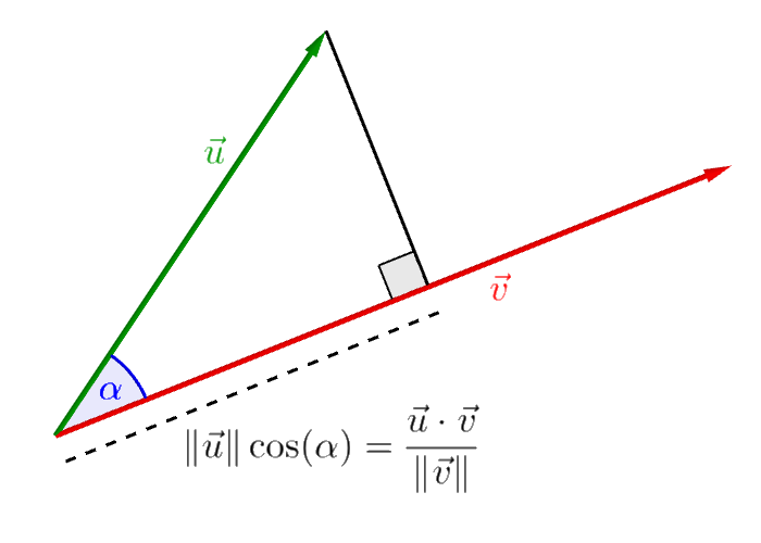
This figure was created with Geogebra and is hereby released to the public domain (CC0 1.0)
. . .
Two vectors are orthogonal, in symbols \(\mathbf{x} \perp \mathbf{y}\), if their dot product is 0.
. . .
The orthogonal projection \(P\mathbf{x}\) of a vector \(\mathbf{x}\) to a subspace \(M \subseteq V\) is determined by \[ \lVert \mathbf{x} - P \mathbf{x} \rVert = \min_{y \in M} \lVert \mathbf{x} - \mathbf{y} \rVert. \]
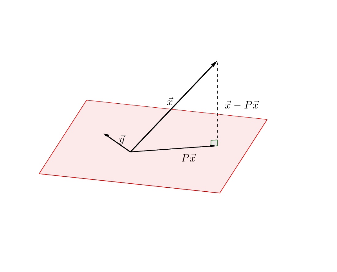
This is often called best approximation property and is equivalent to the relation \[ \langle \mathbf{x} - P \mathbf{x}, \mathbf{y} \rangle = 0 \quad \forall \mathbf{y} \in M. \]
Proof. See [1], Proposition 1.17 (p. 23).
Another useful inequality is the Hölder inequality, a generalization of the Cauchy-Schwarz inequality:
For any vectors \(\mathbf{x}, \mathbf{y}\) and positive numbers \(p, q\) with \(1/p + 1/q = 1\), it is \[ \lvert \langle \mathbf{x}, \mathbf{y} \rangle \rvert \leq \lVert \mathbf{x} \rVert^p + \lVert \mathbf{y} \rVert^q \]
Let \(\{ \mathbf{q}_1, \dotsc, \mathbf{q}_n \}\) be a Orthonormalbasis (ONB) of \(V\). Then each vector \(\mathbf{x} \in V\) possesses a representation of the form \[ \mathbf{x} = \sum_{i=1}^n \langle \mathbf{x}, \mathbf{q}_i \rangle \, \mathbf{q}_i \]
. . .
and there holds the Parseval identity:
\[ \lVert \mathbf{x} \rVert_2^2 = \sum_{i=1}^n \lvert \langle \mathbf{x}, \mathbf{q}_i \rangle \rvert^2 \]
. . .
The Gram-Schmidt-algorithm can be used to construct an ONB from an arbitrary basis:
. . .
Let \(\{\mathbf{v}_1, \dotsc, \mathbf{v}_n\}\) be an arbitrary basis of \(V\). Then the following algorithm results in a ONB \(\{\mathbf{u}_1, \dotsc, \mathbf{u}_n\}\):
\[ \begin{aligned} %\mathbf{u}_1 &= \frac{\mathbf{v}_1}{\lVert \mathbf{v}_1 \rVert}, \\ \widetilde{\mathbf{u}}_k &= \mathbf{v}_k - \sum_{j=1}^{k-1} \frac{\langle \mathbf{v}_k, \mathbf{u}_j \rangle}{ \lVert \mathbf{u}_j \rVert^2} \mathbf{u}_j \\ \mathbf{u}_k &:= \frac{\widetilde{\mathbf{u}}_k}{\lVert \widetilde{\mathbf{u}}_k \rVert} \end{aligned} \]
Linear Operators and Matrices
A mappinng \(\varphi: \mathbb{R}^n \to \mathbb{R}^m\) is called linear, if: \[ \varphi(a\mathbf{x} + b \mathbf{y}) = a \varphi(\mathbf{x}) + b \varphi(\mathbf{y}) \]
We can describe a linear mapping with a matrix \(A\) and the usual rules for matrix-vector multiplication. \[ A = \begin{pmatrix} a_{11} & \dots & a_{1n} \\ \vdots & & \vdots \\ a_{m1} & \dots & a_{mn} \end{pmatrix} , \qquad (A\mathbf{x})_i = \sum_{j=1}^n A_{ij} x_j \]
. . .
A linear operator \(A: X \to Y\) is called bounded, if there is a constant \(C \gt 0\) such that \[ \lVert A \mathbf{x} \rVert_Y \leq C \lVert \mathbf{x} \rVert_X . \]
For any bounded operator we can define the operator norm via \[ \lVert A \rVert := \sup_{\lVert \mathbf{x} \rVert = 1} \lVert A \mathbf{x} \rVert. \] The operator norm is the smalles possible bound and we have \(\lVert A \mathbf{x} \rVert \leq \lVert A \rVert \, \lVert \mathbf{x} \rVert\) for any \(\mathbf{x}\).
For a given a matrix \(A\) we can define the transposed matrix \(A^\intercal\): \[ A^\intercal := \begin{pmatrix} a_{11} & \dots & a_{m1} \\ \vdots & & \vdots \\ a_{1n} & \dots & a_{mn} \end{pmatrix}, \]
A matrix \(A \in \mathbb{R}^{n\times n}\) is called
- symmetric, if \(A^\intercal = A\), and
- orthogonal, if \(A^\intercal A = I\),
- positive definite, if \(\mathbf{x}^\intercal A \mathbf{x} \gt 0 \; \forall \mathbf{x} \in V\).
Orthogonal matrices \(Q\) are the mapping matrices of isomatric transformations, i.e. they do not change the norm of a vector under transformation:
\[ \lVert Q \mathbf{x} \rVert = \lVert \mathbf{x} \rVert \]
This can be seen via: \[ \lVert Q\mathbf{x} \rVert^2 = \langle Q\mathbf{x}, Q\mathbf{x} \rangle = (Q \mathbf{x})^\intercal Q\mathbf{x} = \mathbf{x}^\intercal Q^\intercal Q \mathbf{x} = \lVert \mathbf{x} \rVert^2 \]
We can think of orthogonal transformations as rotations and reflections. For example, \[ Q_\alpha = \begin{pmatrix} 1 & 0 & 0 & 0 & 0 \\ 0 & \cos(\alpha) & 0 & -\sin(\alpha) & 0 \\ 0 & 0 & 1 & 0 & 0 \\ 0 & \sin(\alpha) & 0 & -\cos(\alpha) & 0 \\ 0 & 0 & 0 & 0 & 1 \end{pmatrix} \] is a rotation matrix in the \(\mathbf{x}_i\,\mathbf{x}_j\) plane and angle \(\alpha\).
As already mentioned, a matrix norm can be induced from a given vector norm; in this sense we define \[ \begin{align*} \lVert A \rVert_1 &:= \max_{j=1, \dotsc, n} \sum_{i=1}^n \lvert a_{ij} \rvert, \\ \lVert A \rVert_\infty &:= \max_{i=1,\dotsc,n} \sum_{j=1}^n \lvert a_{ij} \rvert \end{align*} \]
Computing the 2-norm of a matrix is not that simple. As it turns out, it is related to the spectral radius of the matrix: \(\lVert A \rVert_2 = \rho(A)\). However, we can get an upper bound on the 2-norm by using the Frobenius norm.
\[ \lVert A \rVert_2 \leq \lVert A \rVert_F = \sum_{i,j=1}^n \lvert a_{ij} \rvert^2 \]
Show that the matrix norms above are indeed induced by their given vector norms; i.e., show that \[ \sup_{\lVert \mathbf{x} \rVert_\infty = 1} \lVert A \mathbf{x} \rVert_\infty = \max_{i=1,\dotsc,n} \sum_{j=1}^n \lvert a_{ij} \rvert \]
Matrix decompositions
For every matrix \(A \in \mathbb{R}^{n\times n}\) with real Eigenvalues, there exists an orthogonal matrix \(U\) such that \[ U^\intercal A U \] is an upper triangle matrix.
. . .
Proof. The proof is a bit technical. I refer to the standard literature on linear algebra:
- Schur decomposition by Marco Tobago (2021), Lectures on matrix algebra.
- Linear Algebra Done Right by Sheldon Axler, Springer (2025), Theorem 6.38 (p. 204)
As a direct result, we obtain the spectral decomposition for symmetric matrices:
If \(A \in \mathbb{R}^{n \times n}\) is symmetric, then there is an orthogonal matrix \(U\) such that \[ U^\intercal A U = D \] is a diagonal matrix with the Eigenvalues of \(A\) as diagonal entries.
. . .
Proof. (draw on slides)
Note that \(A^\mathrm{T} A\) is symmetric for any matrix A. This means that by applying the previous theorem to \(A^\intercal A\) we can get a generalisation for non-symmetric matrices:
. . .
Let \(A \in \mathbb{K}^{n \times n}\) be arbitrary real or complex. Then, there exist unitary matrices \(V \in \mathbb{K}^{n \times n}\) and \(U \in \mathbb{K}^{m \times m}\) such that \[ A = U \Sigma V^\ast, \quad \Sigma = \mathrm{diag}(\sigma_1, \dotsc, \sigma_p) \in \mathbb{R}^{m \times n}, \quad p = \min(m, n) \] where \(\sigma_1 \geq \sigma_2 \geq \dotso \sigma_p \geq 0\).
Depending on whether \(m \leq n\) or \(m \geq n\) the matrix \(\Sigma\) has the form \[ \left( \begin{array}{ccc|c} \sigma_1 \\ &\ddots & & 0\\ & & \sigma_m \end{array} \right) \qquad \text{or} \quad \left( \begin{array}{ccc} \sigma_1 \\ &\ddots \\ & & \sigma_m \\ \hline & 0 \end{array} \right) \]
. . .
Proof. See Linear Algebra Done Right by Sheldon Axler, Springer (2025), Section 7.E.
. . .
From a visual point of view, the SVD can be thought of as a decomposition into a shear and two rotations.
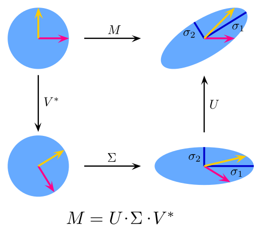
Author: Georg-Johann source: wikimedia.org license: CC BY-SA 3.0
. . .
The Singular value decomposition has applications in machine learning, where it is often used for dimensionality reduction.
. . .
See also: A Singularly Valuable Decomposition: The SVD of a Matrix
Banach fixed-point theorem
An operator \(A: V \to V\) is called a contraction, if there exists a number \(0 \le q \leq 1\) such that \[ \lVert F(\mathbf{x}) - F(\mathbf{y}) \rVert \leq q \lVert \mathbf{x} - \mathbf{y} \rVert. \]