---
title: "Convex Sets and convex Functions"
author: "Marcel Angenvoort"
date: 2025-07-01
#doi: 10.5555/12345678
bibliography: "references.bib"
abstract: >
Lorem ipsum dolor sit amet, consetetur sadipscing elitr, sed diam nonumy eirmod tempor invidunt ut labore et dolore magna aliquyam erat, sed diam voluptua. At vero eos et accusam et justo duo dolores et ea rebum. Stet clita kasd gubergren, no sea takimata sanctus est Lorem ipsum dolor sit amet. Lorem ipsum dolor sit amet, consetetur sadipscing elitr, sed diam nonumy eirmod tempor invidunt ut labore et dolore magna aliquyam erat, sed diam voluptua. At vero eos et accusam et justo duo dolores et ea rebum. Stet clita kasd gubergren, no sea takimata sanctus est Lorem ipsum dolor sit amet.
keywords: ["math", "optimization", "julia", "90-01", "90C30"]
jupyter: julia-1.12
execute:
enabled: true
format:
html:
output-file: convexity.html
revealjs:
output-file: convexity-slides.html
# typst:
# output-file: convexity.pdf
---
Convex Sets
-----------
Before we start with optimisation algorithms, we first need to introduce some concepts.
. . .
:::{.callout-note}
## Convex Set
A set $M$ is called **convex** if for any $\mathbf{x}_1, \mathbf{x}_2 \in M$:
$$
\theta \mathbf{x}_1 + (1-\theta) \mathbf{x}_2 \in M
\qquad \forall \theta \in [0, 1]
$$
:::
. . .
In other words, a set is convex if any line connecting two of its points is also contained within the set.
. . .
::: {.figure layout="[0.4, -0.1, 0.4]" layout-valign="bottom" #fig-examples-convex-nonconvex-set}
 license: [CC BY-SA 4.0](https://creativecommons.org/licenses/by-sa/4.0/)](images/convex_set-wikipedia.svg){width=70%}
 license: [CC BY-SA 4.0](https://creativecommons.org/licenses/by-sa/4.0/)](images/nonconvex_set-wikipedia.svg){width=70%}
Examples for convex and nonconvex sets
:::
---
The expression $\theta \mathbf{x}_1 + (1-\theta) \mathbf{x}_2$ is called an **convex-combination**.
. . .
This can be generalized to more than two points.
Let's say we have multiple points $x_1, \dotsc, x_n$, then we have
$$
\sum_{i=1}^n \theta_i \mathbf{x}_i \in M
$$
where
$$
\theta_i \ge 0 \quad \forall 1 \leq i \leq n, \quad \sum_{i=1}^n \theta_i = 1.
$$
. . .
For anyone familiar with statistics, this will look very similar to the
expectation of a probability distribution.
And indeed, this can be generalised to continuous functions:
Suppose $p(\mathbf{x})$ satisfies $p(\mathbf{x}) \gt 0$ and
$$
\int_M p(\mathbf{x}) \, \mathrm{d}\mathbf{x} = 1,
$$
then
$$
\int_M p(\mathbf{x}) \mathbf{x} \, \mathrm{d}\mathbf{x} \in M.
$$
In other words, the expectation value must be within the convex set.
### Examples for convex sets:
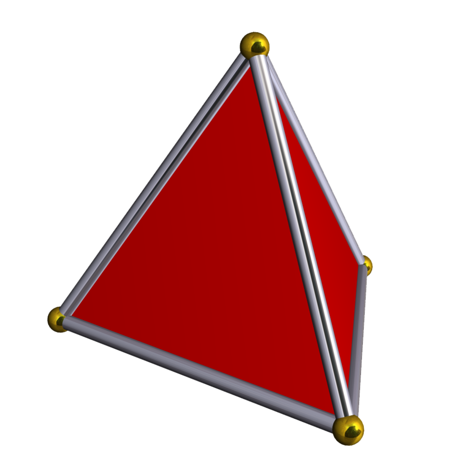
1. Simplices:
$$
S = \left\{
\mathbf{x} \in \mathbb{R}^n: \exists \theta_1, \dotsc, \theta_n \in [0, 1], \, \textstyle\sum_{i=1}^n \displaystyle \theta_i = 1 : \mathbf{x} = \sum_{i=1}^n \theta_i \mathbf{v}_i
\right\}
$$
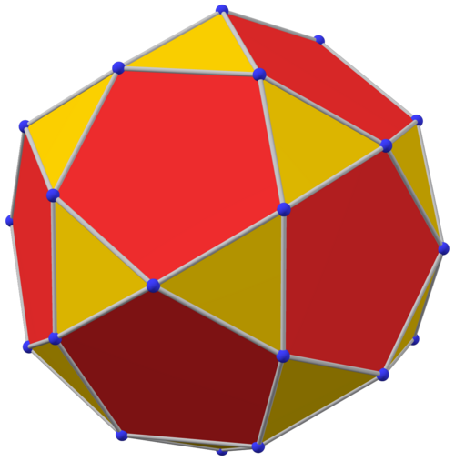
2. Polyhedra
$$
P = \Bigl\{
\mathbf{x} \in \mathbb{R}^n : \mathbf{a}_j^\mathrm{T} \mathbf{x} \leq b_j, \, \mathbf{c}_k^\mathrm{T} \mathbf{x} = d_k, \, j=1,\dotsc, m, \, k=1,\dotsc,p
\Bigr\}
$$
. . .
::: {.figure layout="[0.4, -0.1, 0.4]" layout-valign="bottom" #fig-simplex-and-polyhedron}

url: [Stella software](https://www.software3d.com/Stella.php)](images/Simplex-wikipedia.png){width=70%}

license: [CC BY-SA 4.0](https://creativecommons.org/licenses/by-sa/4.0/)](images/Polyhedron-wikipedia.png){width=70%}
Simplices and Polyhedra are examples for convex sets.
:::
### Operations that preserve Convexity
- **Intersection**:
If $A$ and $B$ are convex,
then the intersection
$$
A \cap B
$$
is also convex.
- **affine Transformations**:
If $M$ is a convex set and $f:\mathbb{R}^n \to \mathbb{R}^n$ is an affine transformation, i.e. $f(\mathbf{x}) = A \mathbf{x} + \mathbf{b}$, then the image
$$
f(M)
$$
is also convex.
- The _projection_ of a convex set onto some of it's coordinates is convex:
If $S \subseteq \mathbb{R}^m \times \mathbb{R}^n$, then
$$
T = \{ x_1 \in \mathbb{R}^m | (x_1, x_2) \in S \;\text{for some $x_2 \in \mathbb{R}^n$} \}
$$
is convex.[@Convex_Optimization_Boyd]
. . .
As a simple corollary, we can see that the perspective function
$f: \mathbb{R}^n \times \mathbb{R}^+$,
$$
f(\mathbf{x}, t) = \frac{\mathbf{x}}{t}
$$
preserves convexity.
. . .
Visually, we can interpret the perspective function as a pinhole camera.
### The Separating Hyperplane Theorem
::: {.callout-important}
## Separating Hyperplane Theorem
Suppose $A$ and $B$ are non-empty, disjoint sets, i.e. $A \cap B = \emptyset$. Then there exists $\mathbf{a} \ne \mathbf{0}$ and $b$ such that
$\mathbf{a}^\mathrm{T} \mathbf{x} \leq b$ for all $\mathbf{x} \in A$ and $b \leq \mathbf{a}^\mathrm{T} \mathbf{x}$ for all $\mathbf{x} \in B$.
:::
. . .

license: [public domain (CC0)](https://creativecommons.org/publicdomain/zero/1.0/)](images/Separating_Hyperplane_Theorem-wikipedia.svg){#fig-separating-hyperplane-theorem .html width="50%"}
. . .
::: {.proof}
See notes.
:::
. . .
::: {.callout-note}
This result can be generalized to the **Hahn-Banach separation theorem**.
:::
Convex Functions
----------------
:::{.callout-note}
## Convex functions
Let $D$ be a convex set. A function $f: D \to \mathbb{R}$ is called **convex** if
$$
f\bigl(\theta \mathbf{x}_1 + (1-\theta) \mathbf{x}_2\bigr) \leq \theta f(\mathbf{x}_1) + (1-\theta) f(\mathbf{x}_2), \qquad \theta \in [0, 1]
$$
:::
. . .
Visually, this means that the graph between two points always lies below the secant line connecting them.
```{julia}
#| label: fig-convex-function
#| fig-cap: A convex function
using Plots
using LaTeXStrings
theme(:dark)
#default(size = (800, 600))  # set default plot size

# Define objective function f
f(x) = -0.01548523*x^4 + 0.09320228*x^3 + 0.21426876*x^2 + -0.83797152*x + 0.90722445

xmin = -0.654
xmax = 4.074
x = range( xmin, xmax, length=100)

x1 = 0.56
x2 = 3.284
theta = 0.3
x_comb = theta * x1 + (1 - theta) * x2

# Plot function f
plot(x, f, color=:darkblue, linewidth=4,
    legend=false,
    xticks = ([x1, x2], ["x₁", "x₂"]),
    yticks = ([f(x1), f(x2)], ["f(x₁)", "f(x₂)"]))

# Draw the line segment connecting (x1, f(x1)) and (x2, f(x2))
plot!([x1, x2], [f(x1), f(x2)],
    lw = 1.5, ls = :dash, color = :green)

# Plot horizontal and vertical lines
plot!([xmin, x1, x1], [f(x1), f(x1), 0],
        lw = 1.5, ls = :dash, color = :gray )
plot!([x2, x2, xmin], [0, f(x2), f(x2)],
    lw = 1.5, ls = :dash, color = :gray )

# Plot points (x1, f(x1)) and (x2, f(x2))
scatter!([x1, x2, x_comb], [f(x1), f(x2), f(x_comb)],
        markersize = 6, color = :red)

# Annotations
annotate!(x_comb + 0.05, f(x_comb) - 0.05, text(L"f(\theta x_1 + (1-\theta) x_2)", :white, :left, :top, 15))
annotate!(x_comb + 0.05, theta * f(x1) + (1-theta) * f(x2), text(L"\theta f(x_1) + (1-\theta) f(x_2)", :white, :right, 15))
```
::: {.hidden}
```{.python}
import numpy as np
import matplotlib.pyplot as plt
plt.style.use('seaborn')

f = lambda x: -0.01548523*x**4 + 0.09320228*x**3 + 0.21426876*x**2 + -0.83797152*x + 0.90722445

xmin = -0.654
xmax = 4.074
x = np.linspace( xmin, xmax, num=100)

x1 = 0.56
x2 = 3.284
theta = 0.55
x_comb = theta * x1 + (1 - theta) * x2

# Plot function f
plt.plot(x, f(x))


# Set xticks and xticklabels
ax = plt.gca()
plt.xticks([x1, x2])
ax.set_xticklabels([r'$x_1$', r'$x_2$'])
plt.yticks(np.array([f(x1), f(x2)]))
ax.set_yticklabels([r'$f(x_1)$', r'$f(x_2)$'])

# move axes to origin
ax.spines["bottom"].set_position("zero")
ax.spines["left"].set_position("zero")

# Box off
ax.spines["top"].set_color("none")
ax.spines["right"].set_color("none")


# Draw the line segment connecting (x1, f(x1)) and (x2, f(x2))
plt.plot([x1, x2], [f(x1), f(x2)],
    color = "green", linestyle = "dashed", linewidth = 1.5)

# Plot horizontal and vertical lines
plt.plot([0, x1, x1], [f(x1), f(x1), 0],
    color = "gray", linestyle = "dashed", linewidth = 1.5)
plt.plot([x2, x2, 0], [0, f(x2), f(x2)],
    color = "gray", linestyle = "dashed", linewidth = 1.5)

# Plot points (x1, f(x1)), (x2, f(x2)) and (xm, f(xm))
plt.plot([x1, x2, x_comb], [f(x1), f(x2), f(x_comb)],
    ".r", markersize = 15)
```
:::
### Examples for convex function
---
Example:
::: {.callout-tip .fragment}
## Himmelblau-function
The [Himmelblau function](https://en.wikipedia.org/wiki/Himmelblau%27s_function) is a common test function for optimization problems.
It is defined by:
$$
f(x,y) = (x^2 + y - 11)^2 + (x + y^2 - 7)^2
$$
This function has four identical local minima, one of which is $f(3, 2) = 0$.
:::
. . .
``` {julia}
#| label: fig-contour-himmelblau
#| fig-cap: Contour plot of the Himmelblau function
using Plots
theme(:dark)

# Himmelblau function
f(x,y) = (x^2 + y - 11)^2 + (x + y^2 - 7)^2

x = range(-5, 5, length=100);
y = range(-5, 5, length=100);
z = @. f(x', y);

contour(x, y, z, levels=20, color=:turbo, cbar=false, lw=1)
scatter!([3.0, -2.805118, -3.779310, 3.584428], [2.0, 3.131312, -3.283186, -1.848126], legend=false)

title!("Contour Plot of the Himmelblau function")
xlabel!("x")
ylabel!("y")
```
::: {.hidden}
``` {julia}
using Plots; plotlyjs()
theme(:dark)

# Himmelblau function
f(x,y) = (x^2 + y - 11)^2 + (x + y^2 - 7)^2

x = range(-5, 5, length=100);
y = range(-5, 5, length=100);
z = @. f(x', y);

surface(x, y, z, color=:hot, cbar=false, lw=1)

title!("Surface Plot of the Himmelblau function")
xlabel!("x")
ylabel!("y")
```
:::
. . .
::: {.callout-tip collapse="true"}
## Solution
Calculate the gradient:
$$
\begin{aligned}
\nabla f &=
\begin{bmatrix}
2(x^2 + y - 11) 2x + 2(x + y^2 - 7) \\
2(x^2 + y - 11) + 2(x + y^2 - 7) 2y
\end{bmatrix} \\
&=
\begin{bmatrix}
4x^3 + 2y^2 + 4xy - 42x - 14 \\
4 y^3 + 2x^2 + 4xy - 26y - 22
\end{bmatrix}
\end{aligned}
$$
Calculate the Hessian:
$$
\begin{aligned}
H &=
\begin{bmatrix}
12x^2 + 4y - 42 & 4x + 4y \\
4x + 4y & 12y^2 + 4x - 26
\end{bmatrix}
\end{aligned}
$$
Substitue $(3, 2)$ for $x$ and $y$:
$$
H(3, 2) =
\begin{bmatrix}
74 & 20 \\
20 & 34
\end{bmatrix}
$$
Determinte the characteristic polynomial:
$$
\begin{aligned}
\det (H - \lambda I) &=
\begin{vmatrix}
74 - \lambda & 20 \\
20 & 34 - \lambda
\end{vmatrix} \\
&= (74 - \lambda) (34 - \lambda) - 20^2 \\
&= \lambda^2 - 108 \lambda + 2116 \\
&\overset{\text{!}}{=} 0
\end{aligned}
$$
Solve for $\lambda$ to obtain the Eigenvalues:
$$
\begin{aligned}
\lambda_1 = \frac{108}{2} - \sqrt{ \left( \frac{108}{2} \right)^2 - 2116}
\approx 25.716 \\
\lambda_2 = \frac{108}{2} + \sqrt{ \left( \frac{108}{2} \right)^2 - 2116}
\approx 82.284
\end{aligned}
$$
All Eigenvalues are greater than 0, so $f$ is in (3, 2) positive definite.
:::
. . .
Alternatively, we can also solve this using the `Symbolics` package in Julia:
::: {.panel-tabset}
## Julia
```{.julia}
using Symbolics
using LinearAlgebra

# Himmelblau function
f(x, y) = (x^2 + y - 11)^2 + (x + y^2 - 7)^2

vars = @variables x, y
f_sym = f(x, y)

H = Symbolics.hessian(f_sym, vars)
H_at_point = substitute.(H, Ref(Dict( x=>3.0, y=>2.0) ))

isposdef(H_at_point)
```
## Python + SymPy
```{.python}
import numpy as np
from sympy import symbols, hessian
from scipy import linalg

f = lambda x, y: (x**2 + y - 11)**2 + (x + y**2 - 7)**2

x, y = symbols("x y")
f_sym = f(x, y)

H = hessian(f_sym, (x,y))
H_at_point = np.array( H.subs( {x:3, y:2} ) )

linalg.cholesky(H_at_point)
```
## MATLAB/Octave
```{.matlab}
pkg load symbolic

% Himmelblau function
f = @(x, y) (x^2 + y - 11)^2 + (x + y^2 - 7)^2

syms x; syms y;

f_sym = f(x, y)
H_sym = hessian(f_sym)
H = function_handle(H_sym)
H_at_point = H(3, 2)

chol(H_at_point)
```
## Python + Autograd
```{.python}
import autograd.numpy as np
from autograd import hessian
from scipy import linalg

f = lambda X: (X[0]**2 + X[1] - 11)**2 + (X[0] + X[1]**2 - 7)**2

H = hessian(f)
point = np.array([3.0, 2.0])
H_at_point = H(point)

linalg.cholesky(H_at_point)
```
:::
---
TODO:
- definition conxex functions
- examples: norm(x), affine fct. f(x) = c.T x + b, quadratic fct. x.T A x
- sublevel sets of convex functions are convex sets (proof trivial)
- Epigraphs: A function is convex if and only if it's epigraph is convex.
- Jennsen's inequality
- Operations that preserve convexity: Composition with affine mapping
- Definition of convex conjugate of a function (generalization of Legendre transformation)
- Examples for convex conjugate (see p. 92)


