---
title: "Introduction"
author: "Marcel Angenvoort"
date: 2025-01-02
#date-modified: 2025-07-01
#doi: 10.5555/12345678
bibliography: "references.bib"
abstract: >
This is a course about Numerical Linear Algebra.
Numerical Linear Algebra is the foundation of modern scientific computing and has many applications: from signal processing to computational physics and data science.
The aim of this course is to give a comprehensive overview of the methods and algorithms used to solve problems such as
linear systems of equations, eigenvalue problems, and matrix decompositions.
I intend to cover iterative methods such as the Jacobi and Gauss-Seidel methods,
as well as advanced techniques for sparse matrices, such as Krylov and multigrid methods.
Furthermore, we will implement the algorithms presented in the programming language Julia.
keywords: ["math", "65Fxx", "numerical linear algebra", "julia"]
jupyter: python3
execute:
enabled: true
format:
html:
output-file: index.html
csl: ../chicago17.csl
revealjs:
output-file: index-slides.html
# typst:
# output-file: introduction.pdf
---
Why learn Numerical Linear Algebra?
-----------------------------------
::: {.notes}
Numerical linear algebra is the foundation of modern scientific computing.
It deals with the numerical approximation of problems such as linear systems and eigenvalue problems.
Many techniques for solving differential equations, such as the finite element method (FEM) or the finite difference method, lead to a system of linear equations;
As such, numerical linear algebra has many applications: from image and signal processing to computational physics, data science and more.
:::
::: {.content-hidden unless-format="revealjs" .fragment}
- Numerical linear algebra is the foundation of scientific computing
- it deals with numerical approximation of linear systems and Eigenvalue problems
- techniques for solving PDEs often lead to a system of linear equations
- many applications: signal processing, computational physics, data science, ...
:::
About this Course
-----------------
::: {.content-visible unless-format="revealjs"}
### Target Audience
This course is primarily aimed at undergraduate students of mathematics, physics and engineering.
However, it is also suitable for engineers who use these algorithms (linear solvers, multigrid methods) in commercial software and want to gain a deeper understanding of how they work.
:::
::: {.content-hidden unless-format="revealjs" }
**Target Audience**:
- Students in math/physics/engineering
- Engineers who want to gain a deeper understanding of numerical algorithms
- anyone who is interested in scientific computing
:::
::: {.content-visible unless-format="revealjs"}
### Prerequisites
This is not a linear algebra course, so a solid understanding of linear algebra is required.
For the implementation of the numerical algorithms, it is also useful to have some programming skills in either MATLAB, Python or Julia.
However, there will be a short introduction to Julia programming at the beginning, so basic programming skills are sufficient.
:::
::: {.content-hidden unless-format="revealjs"}
. . .
**Prerequisites:**
- solid knowledge of Linear Algebra
- basic programming skills (Julia/Python/MATLAB)
:::
::: {.notes .hidden}
**Target Audience**
This course is primarily aimed at undergraduate students of mathematics, physics and engineering.
However, it is also suitable for engineers who use these algorithms (linear solvers, multigrid methods) in commercial software and want to gain a deeper understanding of how they work.
**Prerequisites**
This is not a linear algebra course, so a solid understanding of linear algebra is required.
For the implementation of the numerical algorithms, it is also useful to have some programming skills in either MATLAB, Python or Julia.
However, there will be a short introduction to Julia programming at the beginning, so basic programming skills are sufficient.
:::
### Syllabus
- Week 1 -- 5: Introduction to Julia
- Week 6 -- 10: Algorithms for dense matrices
- Perturbation theory
- Direct solvers for linear systems
- Iterative solvers for linear systems (Gauss-Seidel)
- Calculation of Eigenvalues (power method)
- Week 11 -- 26: Algorithms for sparse matrices
- Sparse LU-decompostion
- Sparse matrix ordering algorithms
- Krylow methods (CG, BiCGStab, GMRES)
- Special iteration methods (multigrid, domain decomposition)
::: {.callout-note .fragment}
The exact structure of this course is subject to change and may vary.
:::
Literature {visibility="hidden"}
--------------------------------
### Theoretical Textbooks
::: {.notes}
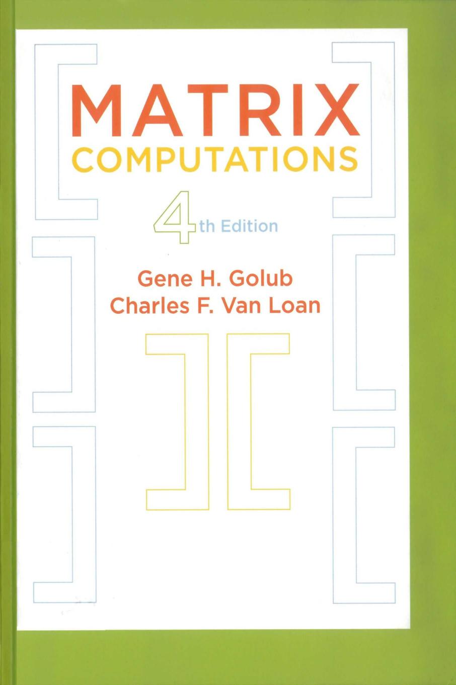
The standard textbook is [@Matrix_Computations_Golub]; it has over [1500 citations](https://zbmath.org/1268.65037) and covers basically everything.
However, it is very dense and not very pleasant to read.
I would recommend it more as a reference book rather than for self study.
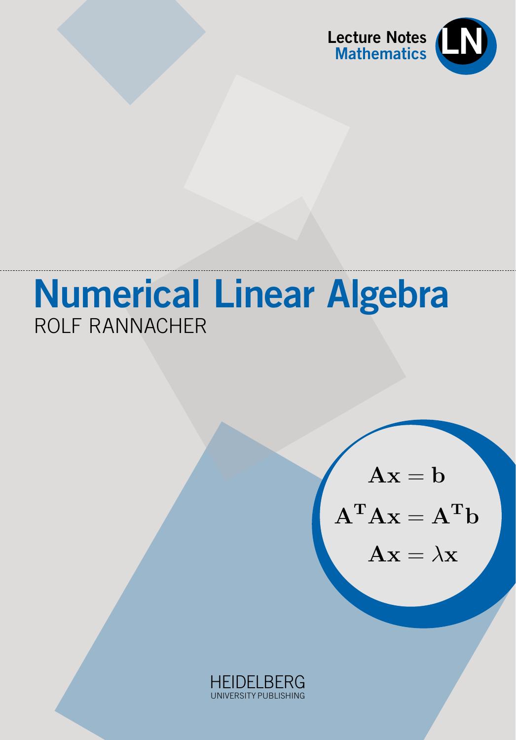
A good alternative is probably [@NumLinAlg_Rannacher], which is very readable and can be used as an introductory textbook. It is open-access.
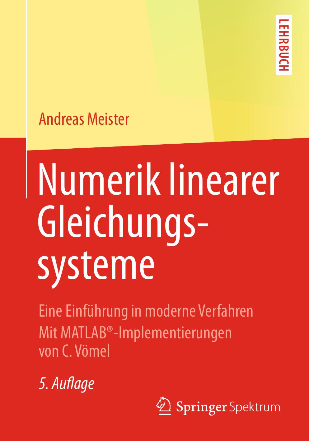
The book [@Numerik_LGS_Meister] is written by a former professor of mine.
It is particularly interesting because it covers advanced Krylow-methods such as [QMRCGSTAB](https://doi.org/10.1137/0915023) and has a large chapter on Multigrid methods.
:::
::: {.figure layout="[0.22, -0.04, 0.22, -0.04, 0.22, -0.04, 0.22]" layout-valign="bottom"}
![[@Matrix_Computations_Golub]](images/literature/Matrix_Computations-Golub.jpg){.fragment}
![[@NumLinAlg_Rannacher]](images/literature/Numerical_Linear_Algebra-Rannacher.jpg){.fragment}
![[@Numerik_LGS_Meister]](images/literature/Numerik_linearer_Gleichungssysteme-Meister.jpg){.fragment}
:::
### Practical Textbooks
::: {.notes}
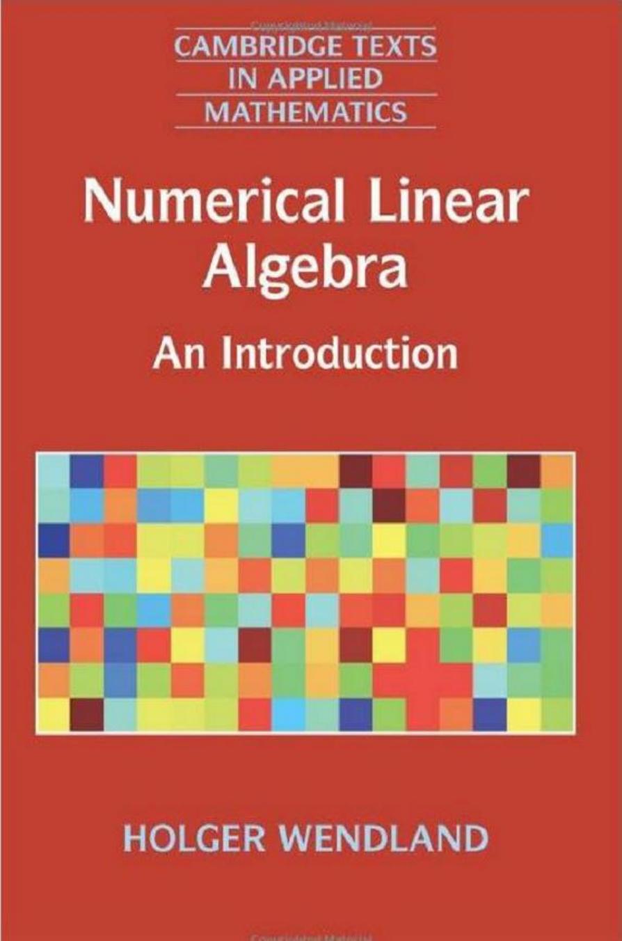
The book [@NumLinAlg_Wendland] is probably the best, in my opinion; it is well structured and has a good balance between theory and application.
The algorithms are given in pseudocode, which makes it easy to implement them in the programming language of your choice.
Since numerical linear algebra is a very practical subject, I think a good book should also include implementations of the actual algorithms.
This is the case for [@NumLinAlg_Matrix_Factorizations], which has code in MATLAB/Octave, and for [@NumLinAlg_Julia], which has implementations in Julia.
The former also has a [companion book](https://link.springer.com/book/10.1007/978-3-030-59789-4) containing many exercises and solutions.
:::
::: {.figure layout="[0.22, -0.04, 0.22, -0.04, 0.22, -0.04, 0.22]" layout-valign="bottom"}
![[@NumLinAlg_Wendland]](images/literature/Numerical_Linear_Algebra-An_Introduction.jpg){.fragment}
![[@NumLinAlg_Matrix_Factorizations]](images/literature/Numerical_Linear_Algebra_and_Matrix_Factorizations.jpg){.fragment}
![[@NumLinAlg_Julia]](images/literature/Numerical_Linear_Algebra_with_Julia-large.jpg){.fragment}
:::
### Advanced Textbooks
::: {.notes}
The books [@Algos_sparse_LinSys] and [@Iterative_Solution] both deal with sparse matrices, but have a very different focus.
While the former covers direct methods and matrix decompositions for developing algebraic preconditioners, the latter deals with advanced iterative methods for sparse systems, such as Krylov, multigrid or domain decomposition methods.
There is also [@Direct_Methods], which is entirely about direct methods for sparse linear systems.
For Eigenvalue problems, there is [@Large_Eigenvalue_Problems], which focuses on Krylov methods, but also covers modern techniques such as AMLS and the Jacobi-Davidson method.
The book is accompanied by MATLAB codes, and has an interesting chapter on applications in physics.
It is probably a good idea to look at some of these books later in this course and focus on individual chapters that are of most interest.
:::
::: {.figure layout="[0.22, -0.04, 0.22, -0.04, 0.22, -0.04, 0.22]" layout-valign="bottom"}
![[@Algos_sparse_LinSys]](images/literature/Algorithms_for_Sparse_Linear_Systems.jpg){.fragment}
![[@Iterative_Solution]](images/literature/Iterative_Solution_of_Large_Sparse_Systems_of_Equations.jpg){.fragment}
![[@Direct_Methods]](images/literature/Direct_Methods_for_Sparse_Linear_Systems.jpg){.fragment}
![[@Large_Eigenvalue_Problems]](images/literature/Numerical_Methods_for_Large_Eigenvalue_Systems.jpg){.fragment}
:::
Introduction
------------
In this course we will study the problem of linear systems of equations
$$
A\mathbf{x} = \mathbf{b},
$$
where $A \in \mathbb{R}^{n \times n}$ is an invertible matrix, $\mathbf{b} \in \mathbb{R}^n$ is a given vector, and $\mathbf{x} \in \mathbb{R}^n$ is the solution that we are looking for.
::: {.content-visible unless-format="revealjs"}
Such systems often come from modelling real-world problems with PDEs that are discretised with an approximation scheme, resulting in a linear system.
As a result, such linear systems can be very large, making it impossible to solve them by hand.
We are therefore interested in finding algorithms that can solve these linear systems efficiently.
However, since we cannot represent real numbers accurately with a computer, such algorithms can only approximate the solution.
Therefore, we also want to estimate the errors that arise from computing the solution numerically.
:::
During the study of numerical methods,
we are interested in the following questions:
1. **Time complexity**: How expensive is the algorithm, i.e. how much time does it take to compute?
2. **Stability/Error estimation**: How does perturbation of the input affect the solution?
3. **Structure**: Can we exploit the structure of the matrix (e.g. symmetric and positive definite)?
4. What if the system is over- or underdetermined, i.e. does not have a unique solution?
Examples for Linear Systems
---------------------------
Linear equations appear almost everywhere.
Here are some examples of applications where such linear systems are used.
See also: [@Numerik_LGS_Meister, chapter 1], [@NumLinAlg_Rannacher, section 0.4] and [@NumLinAlg_Wendland, section 1.1]
1. Partial Differential Equations
------------------------------
The Poisson equation is one of the simplest differential equations.
It describes the electric potential in a capacitor with a given charge density.
$$
\begin{aligned}
- \Delta u &= f, && \text{in $\Omega$}, \\
u &= 0, && \text{on $\partial\Omega$}
\end{aligned}
$$
. . .
Here, $\Omega := [a, b]^2 \subseteq \mathbb{R}^2$ is the domain of the problem, and $u = 0$ is the (Dirichlet) boundary condition.
. . .
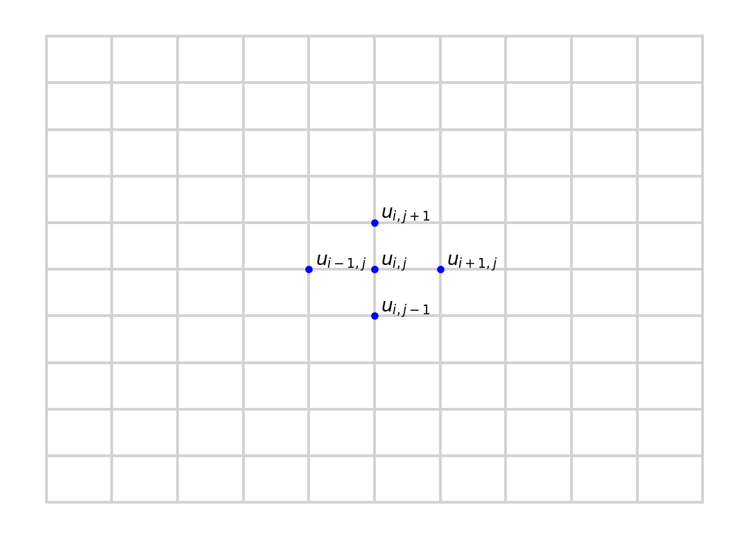
To solve this equation using the finite difference method, we must first discretise the domain.
A simple approach would be to use a regular grid as shown in the figure below.
``` {python}
#| fig-cap: "Regular grid for the Poisson equation"
#
import numpy as np
import matplotlib.pyplot as plt

x = np.linspace(0, 1, num=11)
y = np.linspace(0, 1, num=11)
X, Y = np.meshgrid(x, y)

# Plot the FDM mesh
plt.plot(X, Y, color="lightgray")
plt.plot(X.T, Y.T, color="lightgray")

# Annotations
plt.text(0.41, 0.51, "$u_{i-1,j}$")
plt.text(0.51, 0.51, "$u_{i,j}$")
plt.text(0.61, 0.51, "$u_{i+1,j}$")
plt.text(0.51, 0.41, "$u_{i,j-1}$")
plt.text(0.51, 0.61, "$u_{i,j+1}$")

# Plot stencil
plt.plot([0.4, 0.5, 0.6, 0.5, 0.5], [0.5, 0.5, 0.5, 0.4, 0.6], ".b")

# Remove axes and spines
ax = plt.gca()
ax.spines['top'].set_visible(False)
ax.spines['right'].set_visible(False)
ax.spines['bottom'].set_visible(False)
ax.spines['left'].set_visible(False)

ax.get_xaxis().set_ticks([])
ax.get_yaxis().set_ticks([])
```
. . .
That way, we can approximate the derivatices via
$$
\begin{aligned}
\frac{\partial^2 u}{\partial x^2} (x_i, y_i)
&\approx
\frac{1}{h}
\left(
\frac{u_{i+1, j} - u_{i,j}}{h} - \frac{u_{i,j} - u_{i-1, j}}{h}
\right) \\
&= \frac{1}{h^2} \bigl( u_{i+1, j} - 2 u_{ij} + u_{i-1,j} \bigr)
\end{aligned}
$$
. . .
and for the Laplacian we obtain:
$$
- \Delta u \approx \frac{1}{h^2}
\bigl(
4 u_{i,j} - u_{i+1,j} - u_{i-1, j} - u_{i,j+1} - u_{i,j-1}
\bigr)
$$
. . .
Now we regroup $u$ row-wise into a single vector:
$$
\begin{aligned}
U_1 &:= u_{1,1},
& U_2 &:= u_{1,2},
&\dotsc&
& U_N &:= u_{1,N}, \\
U_{N+1} &:= u_{2, 1},
& U_{N+2} &:= u_{2,2},
&\dotsc&
& U_{N^2} &:= u_{N, N}
\end{aligned}
$$
. . .
This leads to the linear system
$$
A =
\begin{pmatrix}
B & -I \\
-I & \ddots & \ddots \\
& \ddots & \ddots & -I \\
& & -I & B
\end{pmatrix}
\in \mathbb{R}^{N^2 \times N^2}
$$
where
$$
B =
\begin{pmatrix}
4 & -1 \\
-1 & \ddots & \ddots \\
&\ddots &\ddots & -1 \\
& & -1 & 4
\end{pmatrix}
\in \mathbb{R}^{N \times N}
%
\quad \text{and} \quad
%
I =
\begin{pmatrix}
1 \\
& \ddots \\
& & \ddots \\
& & & 1
\end{pmatrix}
$$
. . .
This linear system is _symmetric, positive definite_ and _sparse_.
Linear Regression
-----------------
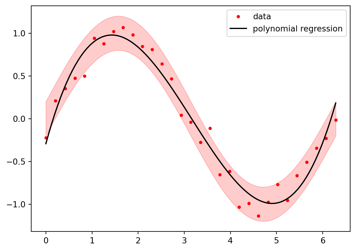
A classic problem in astronomy is the method of least squares, used by Carl Friedrich Gauss to predict the position of the newly discovered asteroid Ceres.
. . .
``` {python}
#| fig-cap: "Polynomial Regression yields in a linear system of equations"
#
import numpy as np
import matplotlib.pyplot as plt

N = 31
sigma = 0.1

# Generate synthetic data
rng = np.random.default_rng(2025)
eps = sigma * rng.standard_normal((N,))
x = np.linspace(0, 2*np.pi, num=N)
y = np.sin(x) + eps

# Compute Polynomial regression (order 3)
p = np.polyfit(x, y, 3)

# Plot data, polyfit and confidence interval
xx = np.linspace(0, 2*np.pi, num=100)
solution = np.sin(xx)
reg_fit = np.polyval(p, xx)

plt.plot(x, y, ".r", label="data")
plt.plot(xx, reg_fit, "k-", label="polynomial regression")
plt.fill_between(xx, solution - 2*sigma, solution + 2*sigma, color="red", alpha=0.2)

plt.legend()
plt.show()
```
. . .
Given $N$ measurements $(x_n, y_n)$, $1 \leq n \leq N$, the goal is to find a function
$$
u(x) = \sum_{k=1}^N c_k x^k
$$
. . .
such that the _mean square error_
$$
E := \left( \sum_{n=1}^N \lvert u(x_n) - y_n \rvert^2 \right)^2
$$
becomes minimal.
. . .
This minimum can be obtained by solving the _normal equation_
$$
A^\top A \mathbf{c} = A^\top \mathbf{y}.
$$
. . .
For the special case of interpolation, this matrix becomes the _Vandermonde_ matrix:
$$
\begin{bmatrix}
1 & x_1 & x_1^2 & \dots & x_1^n \\
1 & x_2 & x_2^2 & \dots & x_2^n \\
1 & x_3 & x_3^2 & \dots & x_3^n \\
\vdots & \vdots & \vdots & \ddots & \vdots \\
1 & x_n & x_n^2 & \dots & x_n^n
\end{bmatrix}
$$
. . .
This is a _full matrix_, meaning each entry is non-zero.
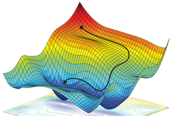
Convex Optimization
-------------------
The example above can be generalised to more general optimisation problems.
Let's say we are given a non-linear objective function $f$ to minimise.
$$
f(x) \overset{\text{!}}{=} \min.
$$
. . .
](images/example_for_optimization.jpg){.fragment}
. . .
Since $f$ is minimal in $x$ implies $f'(x) = 0$, finding the minimum of a convex function is equivalent to finding the roots of it's derivative, so we can use the Newton-Raphson method:
. . .
$$
x_{n+1} = x_n - \alpha \frac{f'(x_n)}{f''(x_n)}
$$
where $\alpha$ is the step size (also called _learning rate_).
. . .
But what if we are dealing with a multi-dimensional optimisation problem?
Then the second derivative of $f$ becomes the Hessian matrix, and the iteration formula is:
. . .
$$
\begin{aligned}
H_f \Delta \mathbf{x} = - \nabla f(\mathbf{x}_n) \\
\mathbf{x}_{n+1} = \mathbf{x}_n + \alpha \Delta \mathbf{x}
\end{aligned}
$$
. . .
This means that with the Newton-Raphson method we have to solve a linear system **for each step**.
## References
::: {#refs}
:::