Introduction

Marcel Angenvoort

2025-01-02

Why learn Numerical Linear Algebra?

Numerical linear algebra is the foundation of modern scientific computing. It deals with the numerical approximation of problems such as linear systems and eigenvalue problems. Many techniques for solving differential equations, such as the finite element method (FEM) or the finite difference method, lead to a system of linear equations; As such, numerical linear algebra has many applications: from image and signal processing to computational physics, data science and more.

• Numerical linear algebra is the foundation of scientific computing
• it deals with numerical approximation of linear systems and Eigenvalue problems
• techniques for solving PDEs often lead to a system of linear equations
• many applications: signal processing, computational physics, data science, …

About this Course

Target Audience:

• Students in math/physics/engineering
• Engineers who want to gain a deeper understanding of numerical algorithms
• anyone who is interested in scientific computing

Prerequisites:

• solid knowledge of Linear Algebra
• basic programming skills (Julia/Python/MATLAB)

Target Audience This course is primarily aimed at undergraduate students of mathematics, physics and engineering. However, it is also suitable for engineers who use these algorithms (linear solvers, multigrid methods) in commercial software and want to gain a deeper understanding of how they work.

Prerequisites This is not a linear algebra course, so a solid understanding of linear algebra is required. For the implementation of the numerical algorithms, it is also useful to have some programming skills in either MATLAB, Python or Julia. However, there will be a short introduction to Julia programming at the beginning, so basic programming skills are sufficient.

Syllabus

• Week 1 – 5: Introduction to Julia
• Week 6 – 10: Algorithms for dense matrices
  • Perturbation theory
  • Direct solvers for linear systems
  • Iterative solvers for linear systems (Gauss-Seidel)
  • Calculation of Eigenvalues (power method)
• Week 11 – 26: Algorithms for sparse matrices
  • Sparse LU-decompostion
  • Sparse matrix ordering algorithms
  • Krylow methods (CG, BiCGStab, GMRES)
  • Special iteration methods (multigrid, domain decomposition)

Note

The exact structure of this course is subject to change and may vary.

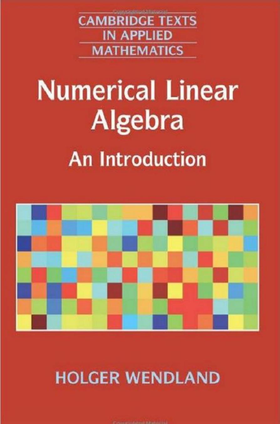
Theoretical Textbooks

The standard textbook is (Golub and Van Loan 2013); it has over 1500 citations and covers basically everything. However, it is very dense and not very pleasant to read. I would recommend it more as a reference book rather than for self study.

A good alternative is probably (Rannacher 2018), which is very readable and can be used as an introductory textbook. It is open-access.

The book (Meister 2015) is written by a former professor of mine. It is particularly interesting because it covers advanced Krylow-methods such as QMRCGSTAB and has a large chapter on Multigrid methods.

(Golub and Van Loan 2013)

 

(Rannacher 2018)

 

(Meister 2015)

 

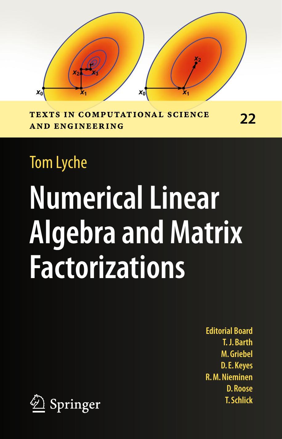
Practical Textbooks

The book (Wendland 2018) is probably the best, in my opinion; it is well structured and has a good balance between theory and application. The algorithms are given in pseudocode, which makes it easy to implement them in the programming language of your choice.

Since numerical linear algebra is a very practical subject, I think a good book should also include implementations of the actual algorithms. This is the case for (Lyche 2020), which has code in MATLAB/Octave, and for (Darve and Wootters 2021), which has implementations in Julia. The former also has a companion book containing many exercises and solutions.

(Wendland 2018)

 

(Lyche 2020)

 

(Darve and Wootters 2021)

 

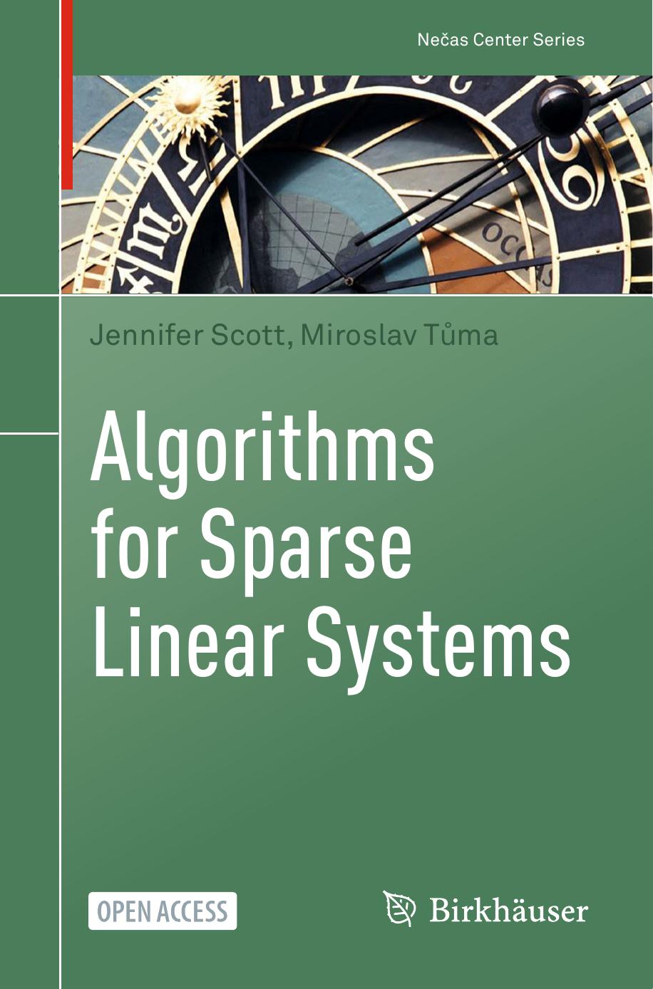
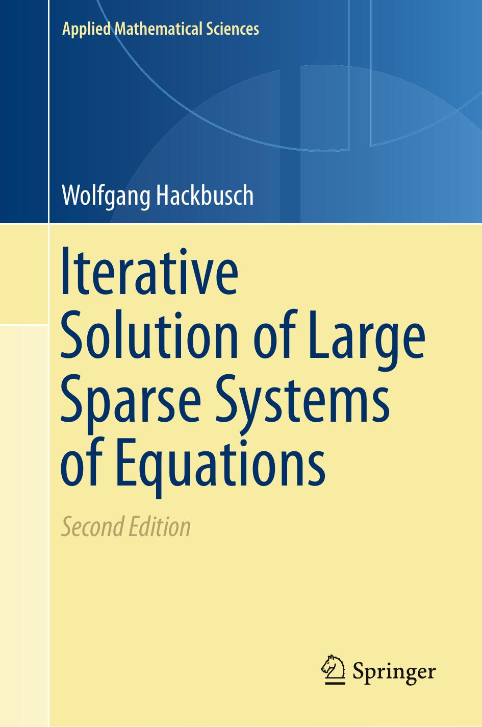
Advanced Textbooks

The books (Scott and Tůma 2023) and (Hackbusch 2016) both deal with sparse matrices, but have a very different focus. While the former covers direct methods and matrix decompositions for developing algebraic preconditioners, the latter deals with advanced iterative methods for sparse systems, such as Krylov, multigrid or domain decomposition methods. There is also (Davis 2006), which is entirely about direct methods for sparse linear systems.

For Eigenvalue problems, there is (Saad 2011), which focuses on Krylov methods, but also covers modern techniques such as AMLS and the Jacobi-Davidson method. The book is accompanied by MATLAB codes, and has an interesting chapter on applications in physics.

It is probably a good idea to look at some of these books later in this course and focus on individual chapters that are of most interest.

(Scott and Tůma 2023)

 

(Hackbusch 2016)

 

(Davis 2006)

 

(Saad 2011)

Introduction

In this course we will study the problem of linear systems of equations \[ A\mathbf{x} = \mathbf{b}, \]

where \(A \in \mathbb{R}^{n \times n}\) is an invertible matrix, \(\mathbf{b} \in \mathbb{R}^n\) is a given vector, and \(\mathbf{x} \in \mathbb{R}^n\) is the solution that we are looking for.

During the study of numerical methods, we are interested in the following questions:

1. Time complexity: How expensive is the algorithm, i.e. how much time does it take to compute?
2. Stability/Error estimation: How does perturbation of the input affect the solution?
3. Structure: Can we exploit the structure of the matrix (e.g. symmetric and positive definite)?
4. What if the system is over- or underdetermined, i.e. does not have a unique solution?

Examples for Linear Systems

Linear equations appear almost everywhere. Here are some examples of applications where such linear systems are used.

See also: (Meister 2015, chap. 1), (Rannacher 2018, sec. 0.4) and (Wendland 2018, sec. 1.1)

1. Partial Differential Equations

The Poisson equation is one of the simplest differential equations. It describes the electric potential in a capacitor with a given charge density.

\[ \begin{aligned} - \Delta u &= f, && \text{in $\Omega$}, \\ u &= 0, && \text{on $\partial\Omega$} \end{aligned} \]

Here, \(\Omega := [a, b]^2 \subseteq \mathbb{R}^2\) is the domain of the problem, and \(u = 0\) is the (Dirichlet) boundary condition.

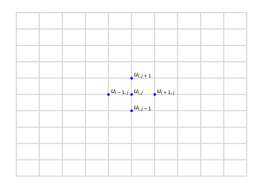
To solve this equation using the finite difference method, we must first discretise the domain. A simple approach would be to use a regular grid as shown in the figure below.

#
import numpy as np
import matplotlib.pyplot as plt

x = np.linspace(0, 1, num=11)
y = np.linspace(0, 1, num=11)
X, Y = np.meshgrid(x, y)

# Plot the FDM mesh
plt.plot(X, Y, color="lightgray")
plt.plot(X.T, Y.T, color="lightgray")

# Annotations
plt.text(0.41, 0.51, "$u_{i-1,j}$")
plt.text(0.51, 0.51, "$u_{i,j}$")
plt.text(0.61, 0.51, "$u_{i+1,j}$")
plt.text(0.51, 0.41, "$u_{i,j-1}$")
plt.text(0.51, 0.61, "$u_{i,j+1}$")

# Plot stencil
plt.plot([0.4, 0.5, 0.6, 0.5, 0.5], [0.5, 0.5, 0.5, 0.4, 0.6], ".b")

# Remove axes and spines
ax = plt.gca()
ax.spines['top'].set_visible(False)
ax.spines['right'].set_visible(False)
ax.spines['bottom'].set_visible(False)
ax.spines['left'].set_visible(False)

ax.get_xaxis().set_ticks([])
ax.get_yaxis().set_ticks([])

Regular grid for the Poisson equation

That way, we can approximate the derivatices via \[ \begin{aligned} \frac{\partial^2 u}{\partial x^2} (x_i, y_i) &\approx \frac{1}{h} \left( \frac{u_{i+1, j} - u_{i,j}}{h} - \frac{u_{i,j} - u_{i-1, j}}{h} \right) \\ &= \frac{1}{h^2} \bigl( u_{i+1, j} - 2 u_{ij} + u_{i-1,j} \bigr) \end{aligned} \]

and for the Laplacian we obtain: \[ - \Delta u \approx \frac{1}{h^2} \bigl( 4 u_{i,j} - u_{i+1,j} - u_{i-1, j} - u_{i,j+1} - u_{i,j-1} \bigr) \]

Now we regroup \(u\) row-wise into a single vector:

\[ \begin{aligned} U_1 &:= u_{1,1}, & U_2 &:= u_{1,2}, &\dotsc& & U_N &:= u_{1,N}, \\ U_{N+1} &:= u_{2, 1}, & U_{N+2} &:= u_{2,2}, &\dotsc& & U_{N^2} &:= u_{N, N} \end{aligned} \]

This leads to the linear system

\[ A = \begin{pmatrix} B & -I \\ -I & \ddots & \ddots \\ & \ddots & \ddots & -I \\ & & -I & B \end{pmatrix} \in \mathbb{R}^{N^2 \times N^2} \]

where

\[ B = \begin{pmatrix} 4 & -1 \\ -1 & \ddots & \ddots \\ &\ddots &\ddots & -1 \\ & & -1 & 4 \end{pmatrix} \in \mathbb{R}^{N \times N} % \quad \text{and} \quad % I = \begin{pmatrix} 1 \\ & \ddots \\ & & \ddots \\ & & & 1 \end{pmatrix} \]

This linear system is symmetric, positive definite and sparse.

Linear Regression

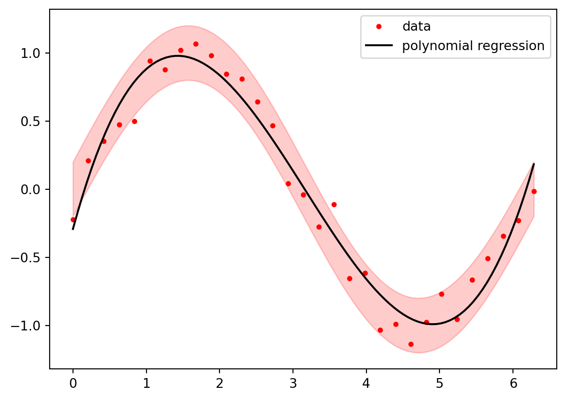
A classic problem in astronomy is the method of least squares, used by Carl Friedrich Gauss to predict the position of the newly discovered asteroid Ceres.

# 
import numpy as np
import matplotlib.pyplot as plt

N = 31
sigma = 0.1

# Generate synthetic data
rng = np.random.default_rng(2025)
eps = sigma * rng.standard_normal((N,))
x = np.linspace(0, 2*np.pi, num=N)
y = np.sin(x) + eps

# Compute Polynomial regression (order 3)
p = np.polyfit(x, y, 3)

# Plot data, polyfit and confidence interval
xx = np.linspace(0, 2*np.pi, num=100)
solution = np.sin(xx)
reg_fit = np.polyval(p, xx)

plt.plot(x, y, ".r", label="data")
plt.plot(xx, reg_fit, "k-", label="polynomial regression")
plt.fill_between(xx, solution - 2*sigma, solution + 2*sigma, color="red", alpha=0.2)

plt.legend()
plt.show()

Polynomial Regression yields in a linear system of equations

Given \(N\) measurements \((x_n, y_n)\), \(1 \leq n \leq N\), the goal is to find a function

\[ u(x) = \sum_{k=1}^N c_k x^k \]

such that the mean square error

\[ E := \left( \sum_{n=1}^N \lvert u(x_n) - y_n \rvert^2 \right)^2 \]

becomes minimal.

This minimum can be obtained by solving the normal equation

\[ A^\top A \mathbf{c} = A^\top \mathbf{y}. \]

For the special case of interpolation, this matrix becomes the Vandermonde matrix:

\[ \begin{bmatrix} 1 & x_1 & x_1^2 & \dots & x_1^n \\ 1 & x_2 & x_2^2 & \dots & x_2^n \\ 1 & x_3 & x_3^2 & \dots & x_3^n \\ \vdots & \vdots & \vdots & \ddots & \vdots \\ 1 & x_n & x_n^2 & \dots & x_n^n \end{bmatrix} \]

This is a full matrix, meaning each entry is non-zero.

Convex Optimization

The example above can be generalised to more general optimisation problems.

Let’s say we are given a non-linear objective function \(f\) to minimise.

\[ f(x) \overset{\text{!}}{=} \min. \]

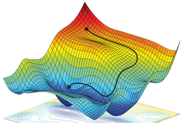
nonlinear optimization
source: arXiv:1805.04829

Since \(f\) is minimal in \(x\) implies \(f'(x) = 0\), finding the minimum of a convex function is equivalent to finding the roots of it’s derivative, so we can use the Newton-Raphson method:

\[ x_{n+1} = x_n - \alpha \frac{f'(x_n)}{f''(x_n)} \]

where \(\alpha\) is the step size (also called learning rate).

But what if we are dealing with a multi-dimensional optimisation problem?
Then the second derivative of \(f\) becomes the Hessian matrix, and the iteration formula is:

\[ \begin{aligned} H_f \Delta \mathbf{x} = - \nabla f(\mathbf{x}_n) \\ \mathbf{x}_{n+1} = \mathbf{x}_n + \alpha \Delta \mathbf{x} \end{aligned} \]

This means that with the Newton-Raphson method we have to solve a linear system for each step.

References

Darve, Eric, and Mary Wootters. 2021. Numerical Linear Algebra with Julia. Philadelphia: Society for Industrial; Applied Mathematics.

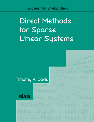
Davis, Timothy A. 2006. Direct Methods for Sparse Linear Systems. SIAM.

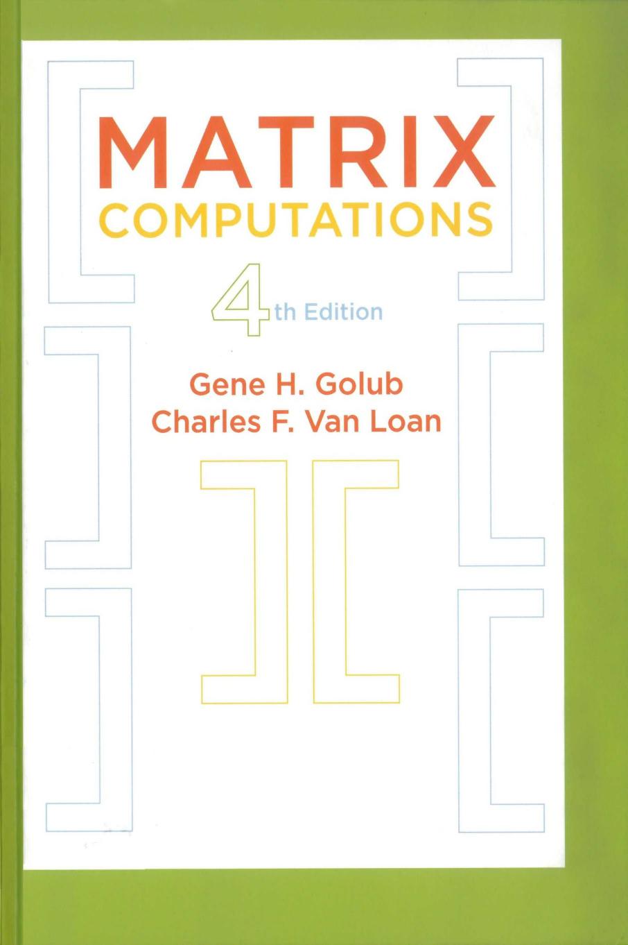
Golub, Gene H., and Charles F. Van Loan. 2013. Matrix Computations. 4th ed. Baltimore, MD: The Johns Hopkins University Press.

Hackbusch, Wolfgang. 2016. Iterative Solution of Large Sparse Systems of Equations. 2nd ed. Springer.

Lyche, Tom. 2020. Numerical Linear Algebra and Matrix Factorizations. Cham, Switzerland: Springer.

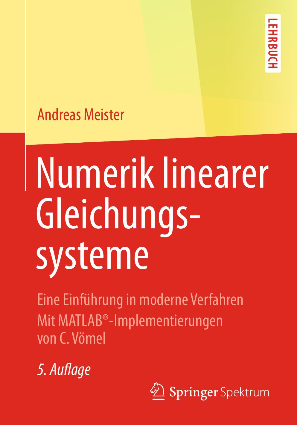
Meister, Andreas. 2015. Numerik linearer Gleichungssysteme. 5th ed. Springer Spektrum.

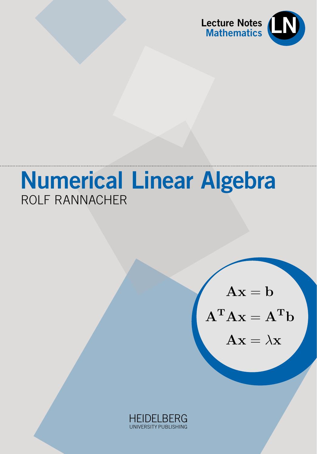
Rannacher, Rolf. 2018. Numerical Linear Algebra. Heidelberg University Publ. https://doi.org/10.17885/heiup.407.

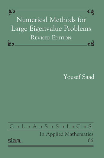
Saad, Yousef. 2011. Numerical Methods for Large Eigenvalue Problems. 2nd ed. SIAM.

Scott, Jennifer, and Miroslav Tůma. 2023. Algorithms for Sparse Linear Systems. Cham, Switzerland: Birkhäuser. https://doi.org/10.1007/978-3-031-25820-6.

Wendland, Holger. 2018. Numerical Linear Algebra: An Introduction. Cambridge University Press.